Melting in spring example

This example simulates the melting of relatively thick sea ice in spring when the sun is shining. We compare bare ice with snow-covered ice to show how snow insulation affects melt rates.

This example demonstrates how to:

• set up a one-dimensional model with multiple grid cells,
• prescribe spatially varying solar insolation,
• use FluxFunction for parameterized heat fluxes,
• add a snow layer with snow_thermodynamics.

Install dependencies

First let's make sure we have all required packages installed.

using Pkg
pkg"add Oceananigans, ClimaSeaIce, CairoMakie"

The physical domain

We generate a one-dimensional grid with 4 grid cells to model different ice columns subject to different solar insolation:

using Oceananigans
using Oceananigans.Units
using ClimaSeaIce
using ClimaSeaIce.SeaIceThermodynamics.HeatBoundaryConditions: RadiativeEmission
using CairoMakie

grid = RectilinearGrid(size=4, x=(0, 1), topology=(Periodic, Flat, Flat))

4×1×1 RectilinearGrid{Float64, Periodic, Flat, Flat} on CPU with 3×0×0 halo
├── Periodic x ∈ [0.0, 1.0) regularly spaced with Δx=0.25
├── Flat y                  
└── Flat z                  

Top boundary conditions

We prescribe different solar insolation values for each grid cell, ranging from -600 to -1200 W m⁻² (negative values indicate downward/into the ice):

solar_insolation = [-600, -800, -1000, -1200] # W m⁻²
solar_insolation = reshape(solar_insolation, (4, 1, 1))

4×1×1 Array{Int64, 3}:
[:, :, 1] =
  -600
  -800
 -1000
 -1200

The ice also emits longwave radiation from its top surface:

outgoing_radiation = RadiativeEmission()

RadiativeEmission(emissivity = Float64, stefan_boltzmann_constant = Float64, reference_temperature = Float64)

Sensible heat flux parameterization

The sensible heat flux from the atmosphere is represented by a FluxFunction. We define the parameters for the bulk formula:

parameters = (
    transfer_coefficient     = 1e-3,  # unitless
    atmosphere_density       = 1.225, # kg m⁻³
    atmosphere_heat_capacity = 1004,  # J kg⁻¹ K⁻¹
    atmosphere_temperature   = -5,    # °C
    atmosphere_wind_speed    = 5      # m s⁻¹
)

(transfer_coefficient = 0.001, atmosphere_density = 1.225, atmosphere_heat_capacity = 1004, atmosphere_temperature = -5, atmosphere_wind_speed = 5)

The flux is positive (cooling by fluxing heat upward away from the upper surface) when the atmosphere temperature is less than the surface temperature:

@inline function sensible_heat_flux(i, j, grid, Tu, clock, fields, parameters)
    Cs = parameters.transfer_coefficient
    ρa = parameters.atmosphere_density
    ca = parameters.atmosphere_heat_capacity
    Ta = parameters.atmosphere_temperature
    ua = parameters.atmosphere_wind_speed
    ℵ  = fields.ℵ[i, j, 1]

    return Cs * ρa * ca * ua * (Tu - Ta) * ℵ
end

aerodynamic_flux = FluxFunction(sensible_heat_flux; parameters)

FluxFunction of sensible_heat_flux (generic function with 1 method) with parameters @NamedTuple{transfer_coefficient::Float64, atmosphere_density::Float64, atmosphere_heat_capacity::Int64, atmosphere_temperature::Int64, atmosphere_wind_speed::Int64}

We combine all top heat fluxes into a tuple:

top_heat_flux = (outgoing_radiation, solar_insolation, aerodynamic_flux)

(RadiativeEmission(emissivity = Float64, stefan_boltzmann_constant = Float64, reference_temperature = Float64), [-600; -800; -1000; -1200;;;], FluxFunction of sensible_heat_flux (generic function with 1 method) with parameters @NamedTuple{transfer_coefficient::Float64, atmosphere_density::Float64, atmosphere_heat_capacity::Int64, atmosphere_temperature::Int64, atmosphere_wind_speed::Int64})

Building the bare-ice model

bare_ice_model = SeaIceModel(grid;
                         ice_consolidation_thickness = 0.05,
                         top_heat_flux)

set!(bare_ice_model, h=1, ℵ=1)

Building the snow-covered model

We add a 20 cm layer of snow on top of the ice. Snow has a much lower thermal conductivity (~0.31 W/m/K) than ice (~2 W/m/K), so it acts as an insulating blanket that reduces the conductive flux through the slab.

snow_thermodynamics = snow_slab_thermodynamics(grid)

snowy_ice_model = SeaIceModel(grid;
                         ice_consolidation_thickness = 0.05,
                         top_heat_flux,
                         snow_thermodynamics)

set!(snowy_ice_model, h=1, ℵ=1, hs=0.2) # 20 cm of snow, no precipitation

Running both simulations

We run both for 30 days with a 10-minute time step, collecting time series for all four columns:

Δt = 10minute

600.0

Bare-ice simulation:

simulation_bare = Simulation(bare_ice_model, Δt=Δt, stop_time=30days)

series_bare = []

function accumulate_bare(sim)
    T = sim.model.ice_thermodynamics.top_surface_temperature
    h = sim.model.ice_thickness
    ℵ = sim.model.ice_concentration
    push!(series_bare, (time(sim),
                        h[1, 1, 1], ℵ[1, 1, 1], T[1, 1, 1],
                        h[2, 1, 1], ℵ[2, 1, 1], T[2, 1, 1],
                        h[3, 1, 1], ℵ[3, 1, 1], T[3, 1, 1],
                        h[4, 1, 1], ℵ[4, 1, 1], T[4, 1, 1]))
end

simulation_bare.callbacks[:save] = Callback(accumulate_bare)
run!(simulation_bare)

[ Info: Initializing simulation...
[ Info:     ... simulation initialization complete (901.106 ms)
[ Info: Executing initial time step...
[ Info:     ... initial time step complete (895.085 ms).
[ Info: Simulation is stopping after running for 2.504 seconds.
[ Info: Simulation time 30 days equals or exceeds stop time 30 days.

Snow-covered simulation:

snowy_ice_simulation = Simulation(snowy_ice_model, Δt=Δt, stop_time=30days)

series_snow = []

function accumulate_snow(sim)
    m  = sim.model
    Tu = m.snow_thermodynamics.top_surface_temperature
    h  = m.ice_thickness
    ℵ  = m.ice_concentration
    hs = m.snow_thickness
    push!(series_snow, (time(sim),
                        h[1, 1, 1], ℵ[1, 1, 1], Tu[1, 1, 1], hs[1, 1, 1],
                        h[2, 1, 1], ℵ[2, 1, 1], Tu[2, 1, 1], hs[2, 1, 1],
                        h[3, 1, 1], ℵ[3, 1, 1], Tu[3, 1, 1], hs[3, 1, 1],
                        h[4, 1, 1], ℵ[4, 1, 1], Tu[4, 1, 1], hs[4, 1, 1]))
end

snowy_ice_simulation.callbacks[:save] = Callback(accumulate_snow)
run!(snowy_ice_simulation)

[ Info: Initializing simulation...
[ Info:     ... simulation initialization complete (161.219 ms)
[ Info: Executing initial time step...
[ Info:     ... initial time step complete (900.525 ms).
[ Info: Simulation is stopping after running for 1.789 seconds.
[ Info: Simulation time 30 days equals or exceeds stop time 30 days.

Extracting the time series

t_bare = [d[1]  for d in series_bare]
h_bare = [[d[3*(c-1)+2] for d in series_bare] for c in 1:4]
ℵ_bare = [[d[3*(c-1)+3] for d in series_bare] for c in 1:4]
T_bare = [[d[3*(c-1)+4] for d in series_bare] for c in 1:4]

t_snow = [d[1]  for d in series_snow]
h_snow  = [[d[4*(c-1)+2] for d in series_snow] for c in 1:4]
ℵ_snow  = [[d[4*(c-1)+3] for d in series_snow] for c in 1:4]
T_snow  = [[d[4*(c-1)+4] for d in series_snow] for c in 1:4]
hs_snow = [[d[4*(c-1)+5] for d in series_snow] for c in 1:4]

4-element Vector{Vector{Float64}}:
 [0.2, 0.19861940380610926, 0.19723880761221851, 0.19585821141832777, 0.19447761522443702, 0.19309701903054627, 0.19171642283665552, 0.19033582664276477, 0.18895523044887402, 0.18757463425498327  …  0.0, 0.0, 0.0, 0.0, 0.0, 0.0, 0.0, 0.0, 0.0, 0.0]
 [0.2, 0.19753067217845546, 0.19506134435691092, 0.19259201653536637, 0.19012268871382182, 0.18765336089227727, 0.18518403307073272, 0.18271470524918818, 0.18024537742764363, 0.17777604960609908  …  0.0, 0.0, 0.0, 0.0, 0.0, 0.0, 0.0, 0.0, 0.0, 0.0]
 [0.2, 0.1964419405508017, 0.19288388110160337, 0.18932582165240505, 0.18576776220320673, 0.1822097027540084, 0.1786516433048101, 0.17509358385561177, 0.17153552440641345, 0.16797746495721513  …  0.0, 0.0, 0.0, 0.0, 0.0, 0.0, 0.0, 0.0, 0.0, 0.0]
 [0.2, 0.1953532089231479, 0.19070641784629577, 0.18605962676944365, 0.18141283569259153, 0.17676604461573941, 0.1721192535388873, 0.16747246246203518, 0.16282567138518306, 0.15817888030833094  …  0.0, 0.0, 0.0, 0.0, 0.0, 0.0, 0.0, 0.0, 0.0, 0.0]

Visualizing the results

set_theme!(Theme(fontsize=18, linewidth=3))

fig = Figure(size=(1200, 1000))

colors = Makie.wong_colors()
labels = ["-600", "-800", "-1000", "-1200"]

4-element Vector{String}:
 "-600"
 "-800"
 "-1000"
 "-1200"

Surface temperature

axT = Axis(fig[1, 1], ylabel="Surface temperature (°C)",
           title="Surface temperature: bare (solid) vs snow-covered (dashed)")
for c in 1:4
    lines!(axT, t_bare ./ day, T_bare[c], color=colors[c], label=labels[c] * " W/m²")
    lines!(axT, t_snow ./ day, T_snow[c], color=colors[c], linestyle=:dash)
end
axislegend(axT, position=:rt)

Makie.Legend()

Ice concentration

axℵ = Axis(fig[2, 1], ylabel="Ice concentration (-)",
           title="Ice concentration: bare (solid) vs snow-covered (dashed)")
for c in 1:4
    lines!(axℵ, t_bare ./ day, ℵ_bare[c], color=colors[c])
    lines!(axℵ, t_snow ./ day, ℵ_snow[c], color=colors[c], linestyle=:dash)
end

Ice thickness

axh = Axis(fig[3, 1], ylabel="Ice thickness (m)",
           title="Ice thickness: bare (solid) vs snow-covered (dashed)")
for c in 1:4
    lines!(axh, t_bare ./ day, h_bare[c], color=colors[c])
    lines!(axh, t_snow ./ day, h_snow[c], color=colors[c], linestyle=:dash)
end

Snow thickness

axs = Axis(fig[4, 1], xlabel="Time (days)", ylabel="Snow thickness (m)",
           title="Snow thickness evolution")
for c in 1:4
    lines!(axs, t_snow ./ day, hs_snow[c], color=colors[c])
end

save("melting_in_spring.png", fig)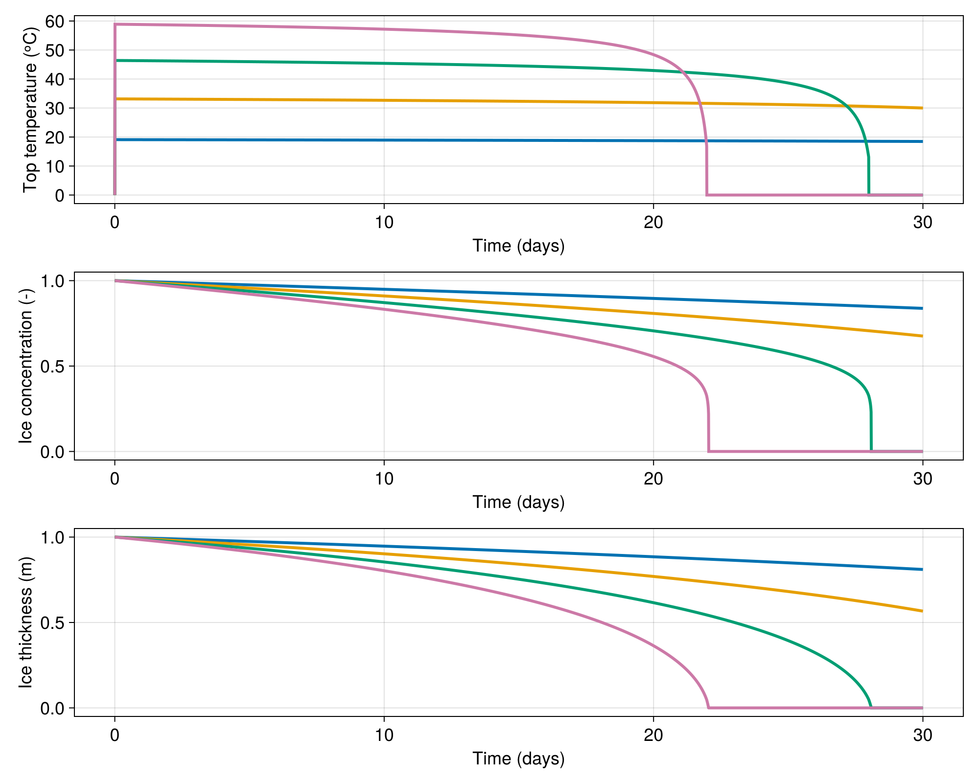

Key observations:

• Snow insulates: snow-covered ice melts more slowly because the low conductivity snow layer reduces the conductive flux.
• Snow melts first: the snow layer disappears before the ice starts melting significantly from the top.
• Warmer surface: the snow surface is warmer than bare ice because the same heat flux produces a larger temperature drop across the more insulating snow+ice slab.

This page was generated using Literate.jl.