This page documents ensemble Kalman inversion (EKI), as well as two variants, ensemble transform Kalman inversion (ETKI) and sparsity-inducing ensemble Kalman inversion (SEKI).
Ensemble Kalman Inversion
What we optimize, and types of solution
One of the ensemble Kalman processes implemented in EnsembleKalmanProcesses.jl is ensemble Kalman inversion (Iglesias et al, 2013). Ensemble Kalman inversion (EKI) is a derivative-free ensemble optimization method that seeks to find the optimal parameters $\theta \in \mathbb{R}^p$ in the inverse problem defined by the data-model relation
\[\tag{1} y = \mathcal{G}(\theta) + \eta ,\]
where $\mathcal{G}$ denotes the forward map, $y \in \mathbb{R}^d$ is the vector of observations and $\eta \in \mathbb{R}^d$ is additive noise. Note that $p$ is the size of the parameter vector $\theta$ and $d$ the size of the observation vector $y$. Here, we take $\eta \sim \mathcal{N}(0, \Gamma_y)$ from a $d$-dimensional Gaussian with zero mean and covariance matrix $\Gamma_y$. This noise structure aims to represent the correlations between observations.
The optimal parameters $\theta^* \in \mathbb{R}^p$ (Maximum Likelihood Estimation) given relation (1) minimize the loss
\[\mathcal{L}(\theta, y) = \frac{1}{2} \left(y - \mathcal{G}(\theta)\right)^{\top} \Gamma_y^{-1} \left(y - \mathcal{G}(\theta) \right),\]
which can be interpreted as the negative log-likelihood given a Gaussian likelihood.
- This is acheived using process
Inversion()and stepping to algorithm time $T=\infty$. This form uses the prior like an initial condition.
If we using a prior to seek a Bayesian solution to our problem, (not just as initialization) then the optimal parameters $\theta^* \in \mathbb{R}^p$ (Maximum A Posteriori estimation) given relation (1) minimize the loss
\[\mathcal{L}(\theta, y) = \frac{1}{2} \left(y - \mathcal{G}(\theta)\right)^{\top} \Gamma_y^{-1} \left(y - \mathcal{G}(\theta) \right) + \frac{1}{2}(\theta - m)^{\top} C^{-1}(\theta-m)\]
which can be interpreted as the negative log-likelihood given a Gaussian likelihood and Gaussian prior $N(m,C)$. This is acheived in two ways:
- using process
Inversion()and terminating the iterations at algorithm time $T=1$ (default), "finite-time variant" - using process
Inversion(prior)and stepping to $T=\infty$. "infinite-time variant"
See how these behave here
The EKI update
Denoting the parameter vector of the $j$-th ensemble member at the $n$-th iteration as $\theta^{(j)}_n$, its update equation from $n$ to $n+1$ under EKI is
\[\tag{2} \theta_{j+1}^{(n)} = \theta_j^{(n)} + \Delta t C^{\theta\mathcal{G}}_j(\Gamma_y + \Delta t C_j^{\mathcal{GG}})^{-1}(y - \mathcal{G}(\theta_j^{(n)})).\]
Where the notations for means and covariances are given as
\[\begin{aligned} C^{\theta\mathcal{G}}_j &= \frac{1}{N}\sum_{n=1}^N \left[ (\theta^{(n)}_j - \overline{\theta_j})\otimes(\mathcal{G}(\theta^{(n)}_j) - \overline{ \mathcal{G}(\theta)}_j) \right],\\ C^{\mathcal{GG}}_j &= \frac{1}{N}\sum_{n=1}^N \left[(\mathcal{G}(\theta^{(n)}_j) - \overline{ \mathcal{G}(\theta)}_j)\otimes(\mathcal{G}(\theta^{(n)}_j) - \overline{ \mathcal{G}(\theta)}_j) \right],\\ \overline{\theta}_j &= \frac{1}{N}\sum_{n=1}^N \theta^{(n)}_j,\qquad \overline{\mathcal{G}(\theta)}_j = \frac{1}{N} \sum_{n=1}^N\mathcal{G}(\theta^{(n)}_j),\\ \end{aligned}\]
There is no difference between the Inversion() and Inversion(prior) updates, but the latter works with an augmented state (see here). The algorithmic timestep (a.k.a learning rate) $\Delta t$ is usually taken to be adaptive with a schedule, as described here.
The final estimate $\bar{\theta}_{N_{\rm it}}$ is taken to be the ensemble mean at the final iteration,
\[\bar{\theta}_{N_{\rm it}} = \dfrac{1}{J}\sum_{k=1}^J\theta_{N_{\rm it}}^{(k)}.\]
For typical applications, a near-optimal solution $\theta$ can be found after as few as 10 iterations of the algorithm, or $10\cdot J$ evaluations of the forward model $\mathcal{G}$. The rules of thumb of choosing $J$ are see here, and to reduce errors when $J \ll p$ , we have sampling-error-correction (localization) approaches here.
Constructing the Forward Map
The forward map $\mathcal{G}$ maps the space of unconstrained parameters $\theta \in \mathbb{R}^p$ to the space of outputs $y \in \mathbb{R}^d$. In practice, the user may not have access to such a map directly. Consider a situation where the goal is to learn a set of parameters $\phi$ of a dynamical model $\Psi: \mathbb{R}^p \rightarrow \mathbb{R}^o$, given observations $y \in \mathbb{R}^d$ and a set of constraints on the value of $\phi$. Then, the forward map may be constructed as
\[\mathcal{G} = \mathcal{H} \circ \Psi \circ \mathcal{T}^{-1},\]
where $\mathcal{H}: \mathbb{R}^o \rightarrow \mathbb{R}^d$ is the observation map and $\mathcal{T}$ is the transformation map from constrained to unconstrained parameter spaces, such that $\mathcal{T}(\phi) = \theta$. A family of standard transformation maps and their inverse are available in the ParameterDistributions module.
Creating the EKI Object
An ensemble Kalman inversion object can be created using the EnsembleKalmanProcess constructor by specifying the Inversion() process type.
The EnsembleKalmanProcess then is built with and initial ensemble, observation and the process. The following utilities describe this
using EnsembleKalmanProcesses # for `construct_initial_ensemble`, `Inversion`, `Observation`
using EnsembleKalmanProcesses.ParameterDistributions # for `constrained_gaussian`

prior = constrained_gaussian("4d-unit-gauss", 0.0, 1.0, -Inf, Inf, repeats=4)

J = 50  # number of ensemble members
initial_ensemble = construct_initial_ensemble(prior, J) # Initialize ensemble from prior (unconstrained u-space)

# data
ydim = 5
y = ones(ydim)
cov_y = 0.01*I

# basic EKI, finite-time
ekiobj = EnsembleKalmanProcess(initial_ensemble, y, obs_noise_cov, Inversion())

# fancier observation container, infinite-time, verbose i/o
y_obs = Observation(
    Dict(
        "samples" => y,
        "covariances" => cov_y,
        "names" => "descriptive_name",
        "metadata" => "some imporant information"
    ),
)

ekiobj = EnsembleKalmanProcess(initial_ensemble, y_obs, Inversion(prior), verbose=true)
See the Prior distributions section to learn about the construction of priors in EnsembleKalmanProcesses.jl. See the Observations section to learn about more complex observation construction and minibatching utilities. Note that the initial ensemble is in the unconstrained u space, apply transform_unconstrained_to_constrained(prior, initial_ensemble) to see the resulting constrained parameter ensemble.
Updating the Ensemble
Once the ensemble Kalman inversion object ekiobj has been initialized, any number of updates can be performed using the inversion algorithm.
A call to the inversion algorithm can be performed with the update_ensemble! function. This function takes as arguments the ekiobj and the evaluations of the forward map at each member of the current ensemble. The update_ensemble! function then stores the new updated ensemble and the inputted forward map evaluations in ekiobj.
A typical use of the update_ensemble! function given the ensemble Kalman inversion object ekiobj, the dynamical model Ψ and the observation map H is
# Given:
# Ψ (some black box simulator)
# H (some observation of the simulator output)
# prior (prior distribution and parameter constraints)

N_iter = 20 # Number of steps of the algorithm

for n in 1:N_iter
    ϕ_n = get_ϕ_final(prior, ekiobj) # Get current ensemble in constrained "ϕ"-space
    G_n = [H(Ψ(ϕ_n[:, i])) for i in 1:J]
    g_ens = hcat(G_n...) # Evaluate forward map
    update_ensemble!(ekiobj, g_ens) # Update ensemble
end
In the previous update, note that the parameters stored in ekiobj are given in the unconstrained Gaussian space where the EKI algorithm is performed. The map $\mathcal{T}^{-1}$ between this unconstrained space and the (possibly constrained) physical space of parameters is encoded in the prior object. The dynamical model Ψ accepts as inputs the parameters in (possibly constrained) physical space, so it is necessary to use the getter get_ϕ_final which applies transform_unconstrained_to_constrained to the ensemble. See the Prior distributions section for more details on parameter transformations.
Solution
The EKI algorithm drives the initial ensemble, sampled from the prior, towards the support region of the posterior distribution. The algorithm also drives the ensemble members towards consensus. The optimal parameter θ_optim found by the algorithm is given by the mean of the last ensemble (i.e., the ensemble after the last iteration),
θ_optim = get_u_mean_final(ekiobj) # optimal parameterTo obtain the optimal value in the constrained space, we use the getter with the constrained prior as input
ϕ_optim = get_ϕ_mean_final(prior, ekiobj) # the optimal physical parameter valueInversion() vs Inversion(prior)
Deeper description of these algorithms is discussed in detail in, for example, Section 4.5 of Calvello, Reich, Stuart). Finite-time algorithms have also been called "transport" algorithms, and infinite-time algorithms are also known as prior-enforcing, or Tikhonov EKI Chada, Stuart, Tong.
Thus far, we have presented the finite-time algorithm Inversion(). The infinite-time variant Inversion(prior) algorithm has two key practical distinctions.
- The initial distribution does not need to come from the prior.
- The particle distribution mean converges to the maximum a-posteriori estimator as $T\to \infty$ (not via an early-termination condition)
Both implementations perform the same update; but in the infinite-time variant, the forward-map, data and noise-covariance are augmented by a Gaussian prior $N(m,C)$ by working with the following:
\[\tilde{\mathcal{G}}(\theta) = [ \mathcal{G}(\theta), \theta] \qquad \tilde{y} = \left[ y, m \right]^{\top}, \qquad \tilde{\Gamma}_y = \begin{bmatrix} \Gamma_y & 0 \\ 0 & C \end{bmatrix}\]
It is implemented as follows (here, for three parameters)
using EnsembleKalmanProcesses
using EnsembleKalmanProcesses.ParameterDistributions
# given `y` `obs_noise_cov` and `prior`

J = 50  # number of ensemble members
initial_dist = constrained_gaussian("not-the-prior", 0, 1, -Inf, Inf, repeats=3)
initial_ensemble = construct_initial_ensemble(inital_dist, J) # Initialize ensemble from prior

ekiobj = EnsembleKalmanProcess(initial_ensemble, y, obs_noise_cov, Inversion(prior))
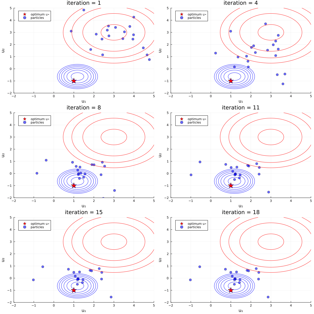
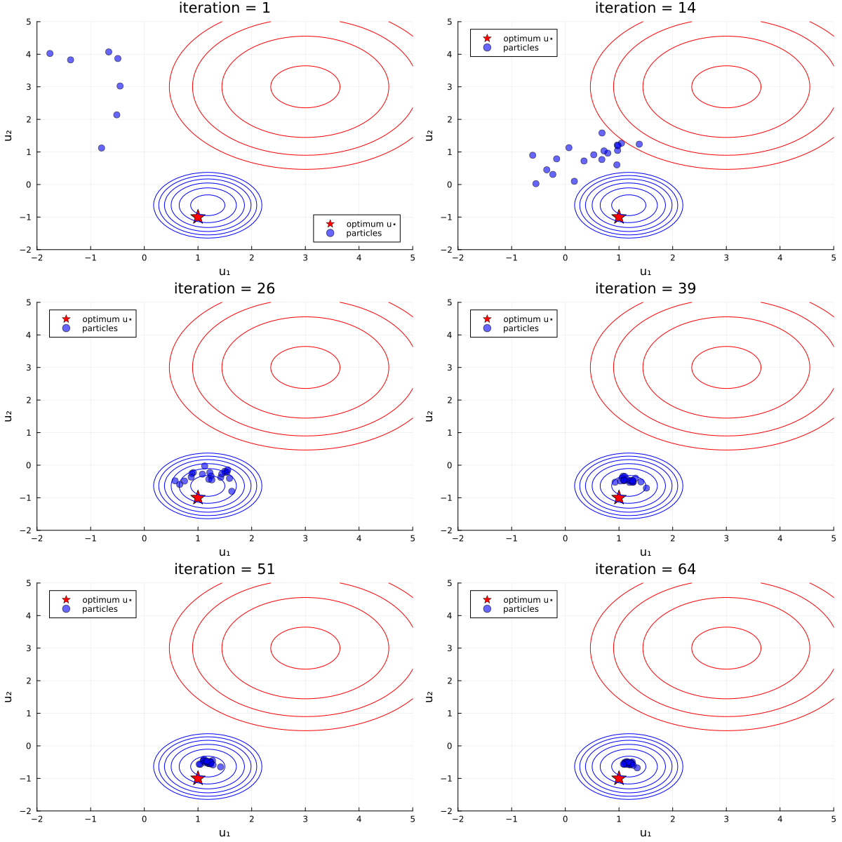
One can see this in-action with the finite- vs infinite-time comparison example here, which was used to produce the plots below:
Left: Inversion (finite-time), Right: Inversion(prior) (infinite-time, initialized off-prior)


Comparative behaviour.
- Initialization:
Inversion()must be initialized from the prior,Inversion(prior)can still find the posterior when initialized off-prior. This might be useful when the prior is very broad and can enter, for example, regions of instability of the users forward model - Prior information:
Inversion()only contains prior information due to its initialization,Inversion(prior)enforces the prior at every iteration. - Solution:
Inversion()terminated at $T=1$ (implemented by default) obtains an accurate MAP estimate, the ensemble spread at exactly $T=1$ can represent a snapshot of the true (Gaussian-approximated) uncertainty.Inversion(prior)obtains this in the limit $T\to\infty$, and undergoes collapse providing no uncertainty information. - Trust in prior
Inversion(), when iterated beyond $T=1$ will lose prior information and thus move to find the MLE (minimize the data-misfit only) at $T\to\infty$, this behaviour might be useful if the prior information is missprecified. - Efficiency:
Inversion()is more efficient thatInversion(prior)as enforcing the prior in the infinite-time algorithm is performed via extending the linear systems to be solved. Performance is also impacted (positively or negatively) by the choice of initial distribution in theInversion(prior)
One can learn more about the early termination for finite-time algorithms here.
Output-scalable variant: Ensemble Transform Kalman Inversion
Ensemble transform Kalman inversion (ETKI) is a variant of EKI based on the ensemble transform Kalman filter (Bishop et al., 2001). It is a form of ensemble square-root inversion, and an implementation can be found in Huang et al., 2022. The main advantage of ETKI over EKI is that it has better scalability as the observation dimension grows: while the naive implementation of EKI scales as $\mathcal{O}(p^3)$ in the observation dimension $p$, ETKI scales as $\mathcal{O}(p)$. This, however, refers to the online cost. ETKI may have an offline cost of $\mathcal{O}(p^3)$ if $\Gamma$ is not easily invertible; see below.
The major disadvantage of ETKI is that it cannot be used with localization or sampling error correction.
ETKI requires storing and inverting the observation noise covariance, $\Gamma^{-1}$. Without care, this can be prohibitively expensive. To this end, we have tools and an API for creating and using scalable or compact representations of covariances that are necessary for scalability. See here for details and examples.
Using ETKI
An ETKI struct can be created using the EnsembleKalmanProcess constructor by specifying the TransformInversion process type:
using EnsembleKalmanProcesses
# given the prior distribution `prior`, data `y` and covariance `obs_noise_cov`,

J = 50  # number of ensemble members
initial_ensemble = construct_initial_ensemble(prior, J) # Initialize ensemble from prior

etkiobj = EnsembleKalmanProcess(initial_ensemble, y, obs_noise_cov,
                               TransformInversion())
The rest of the inversion process is the same as for regular EKI.
Sparsity-Inducing Ensemble Kalman Inversion
We include Sparsity-inducing Ensemble Kalman Inversion (SEKI) to add approximate $L^0$ and $L^1$ penalization to the EKI (Schneider, Stuart, Wu, 2020).