Insolation Examples
This page demonstrates various use cases of Insolation.jl through visualizations and practical examples. These examples show how to calculate and visualize solar radiation patterns across different timescales and locations.
Diurnal Cycle of Insolation
The diurnal cycle shows how insolation and solar zenith angle vary throughout a day at a specific location. This is useful for understanding the daily energy input and for applications such as solar power forecasting.
Pasadena in Winter: Clear diurnal cycle with peak insolation at solar noon. The solar zenith angle reaches its minimum of about 56° at midday (the midwinter noon sun stands only about 34° above the horizon at this latitude). At night the plotted zenith angle saturates at 90°, because it is reconstructed from the returned $\mu = \cos\theta$, which the package clamps to zero when the sun is below the horizon.
using Insolation
using Dates

include("plot_diurnal_cycle.jl")

# Load orbital data
od = OrbitalDataSplines()

# Example 1: Pasadena, California in January (mid-latitude winter)
lat, lon = [34.15, -118.14]  # Pasadena coordinates
date = DateTime(2020, 01, 10)
# `timezone` is the offset added to local time to obtain UTC.
timezone = +8  # Pacific Standard Time is UTC-8, so add 8 h to get UTC
diurnal_cycle(lat, lon, date, od, timezone, "Pasadena_January.png")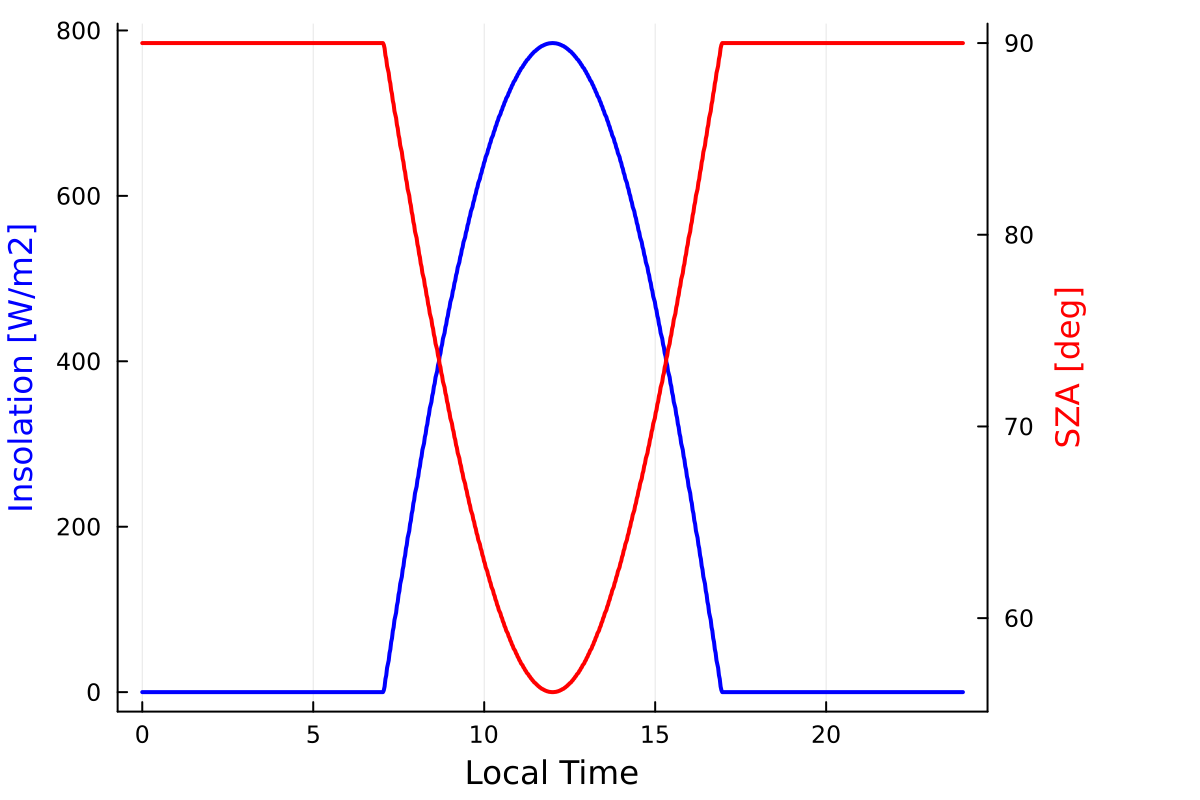
Finland in Summer: Rovaniemi lies a few kilometers south of the Arctic Circle (at 66.56°N, where the sun first stops setting at summer solstice), so at solstice the sun just grazes the horizon at solar midnight: the computed insolation touches zero only for about half an hour. The sustained insolation through the night hours is the "midnight sun". Note that both the midday maximum and the midnight minimum fall more than an hour after 12:00 and 0:00 on the clock, because Eastern European Summer Time runs well ahead of local solar time at this longitude. (In reality, atmospheric refraction keeps the midnight sun visible even slightly south of the Arctic Circle; this package computes the geometric solar position without refraction.)
# Example 2: Rovaniemi, Finland in June (Arctic summer - midnight sun)
lat, lon = [66.50, 25.73]  # Rovaniemi coordinates (just south of the Arctic Circle)
date = DateTime(2020, 06, 20)  # Summer solstice
# `timezone` is the offset added to local time to obtain UTC.
timezone = -3  # Eastern European Summer Time is UTC+3, so subtract 3 h to get UTC
diurnal_cycle(lat, lon, date, od, timezone, "Finland_June.png")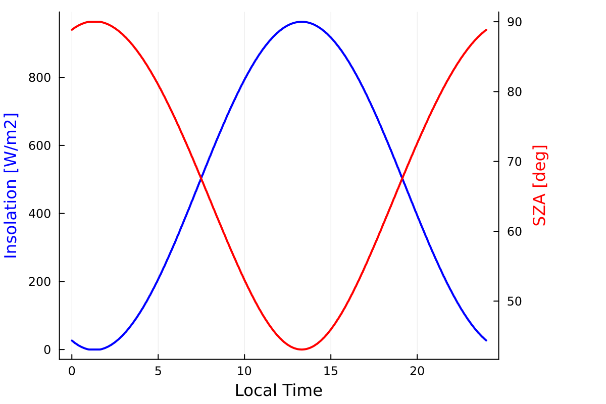
Latitudinal and Seasonal Variations
The following examples show how daily-averaged insolation varies with latitude and day of year, revealing Earth's seasonal cycles and the role of orbital parameters.
Modern Climate (J2000 Epoch)
import Insolation
import Insolation.Parameters as IP
import ClimaParams as CP

FT = Float64
param_set = IP.InsolationParameters(FT)

include("plot_insolation.jl")

# Get current epoch orbital parameters
γ0 = IP.obliq_epoch(param_set)
ϖ0 = IP.lon_perihelion_epoch(param_set)
e0 = IP.eccentricity_epoch(param_set)
od = Insolation.OrbitalDataSplines()

# Calculate daily-mean insolation across latitudes and days
days, lats, F0 = calc_day_lat_insolation(od, 365, 180, param_set)
plot_day_lat_insolation(days, lats, F0, "YlOrRd", title, "insol_example1.png")
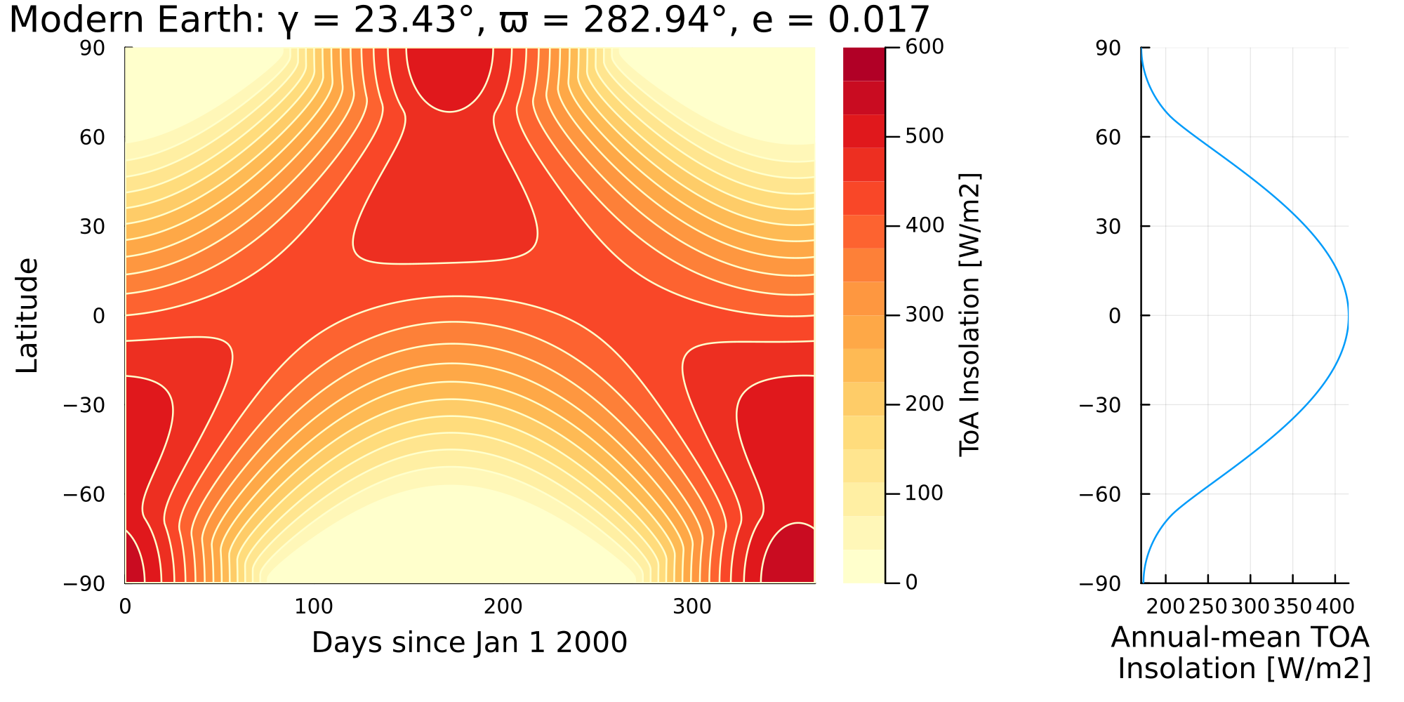
This plot shows daily-averaged TOA insolation as a function of latitude and day of year for modern Earth (J2000 epoch). Key features:
- Solstices: The maximum occurs at the summer pole (June in the NH, December in the SH), where continuous polar day outweighs the low solar elevation. This holds for any obliquity above about 20.7°; below that the maximum lies at an intermediate latitude.
- Equinoxes: Insolation is symmetric about the equator around March 20 and September 22, when day and night are equally long everywhere.
- Asymmetry between the solstices: December insolation is the more intense of the two, because perihelion currently falls in early January, near southern summer solstice.
- Annual mean: The right panel shows the latitudinal gradient, decreasing monotonically and almost symmetrically away from the equator. Annual-mean insolation at the equator is more than twice that at the poles (about 416 versus 172 W/m²).
Effect of Reduced Obliquity
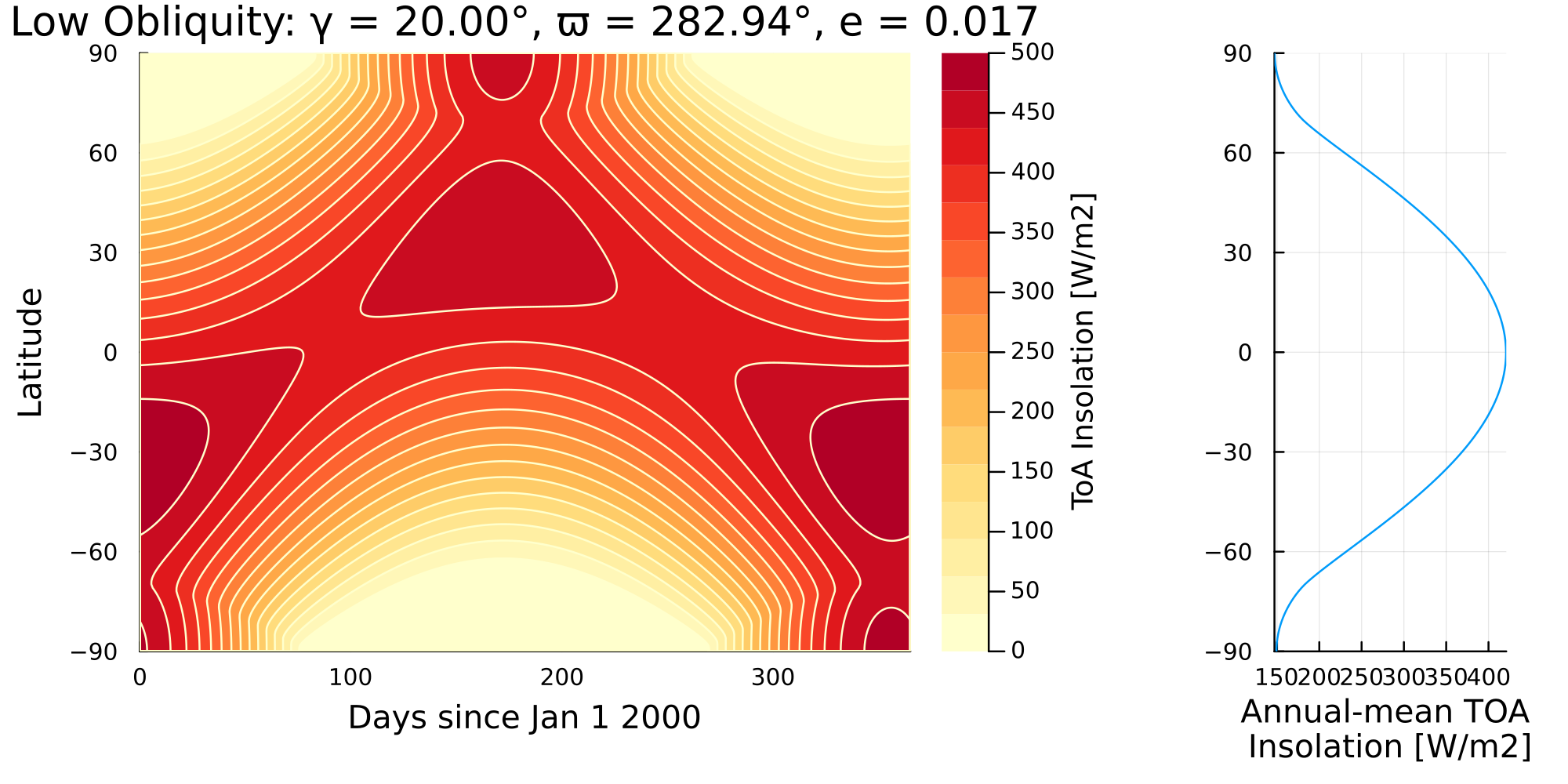
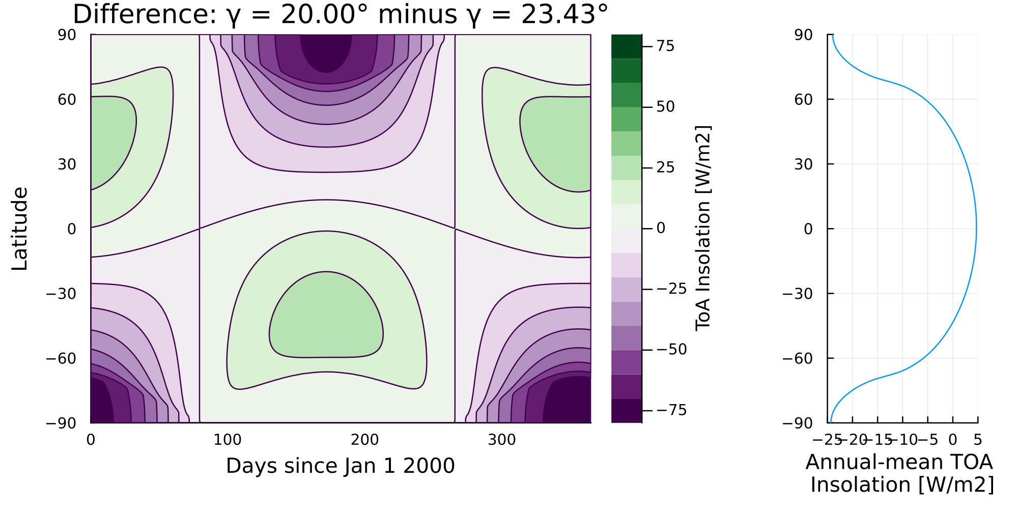
Obliquity (axial tilt) controls the strength of seasonal cycles. Here we reduce obliquity from its present value to 20° to demonstrate its impact; the figure titles report the values actually used.
# Reduce obliquity to 20.0° (from Earth's present value of about 23.4°)
param_set_low_obliq = IP.InsolationParameters(FT, (; obliq_epoch = deg2rad(20.0)))
γ1 = IP.obliq_epoch(param_set_low_obliq)
days, lats, F2 = calc_day_lat_insolation(od, 365, 180, param_set_low_obliq)

plot_day_lat_insolation(days,lats,F2,"YlOrRd",  title, "insol_example2a.png")
plot_day_lat_insolation(days, lats, F2-F0, "PRGn", title, "insol_example2b.png")
Absolute Insolation (top): With reduced obliquity, polar regions receive less summer insolation, and the tropical regions receive slightly more year-round.
Difference Plot (bottom): purple is a decrease, green an increase. Reducing obliquity:
- Decreases summer insolation at middle and high latitudes, by up to 80 W/m² at the summer pole, and in the annual mean by 25 W/m² at the poles
- Increases insolation slightly in the tropics and in the winter hemisphere outside polar night
- Results in weaker seasonal cycles in both hemispheres, symmetrically
Because obliquity changes the annual-mean insolation at a given latitude — unlike precession, which does not — it directly alters the equator-to-pole gradient that drives the atmospheric and oceanic circulation. Lower obliquity means milder seasons and a steeper annual-mean gradient, which matters for Earth's past climates and for other planets alike.
Extreme Obliquity (Uranus-like Configuration)
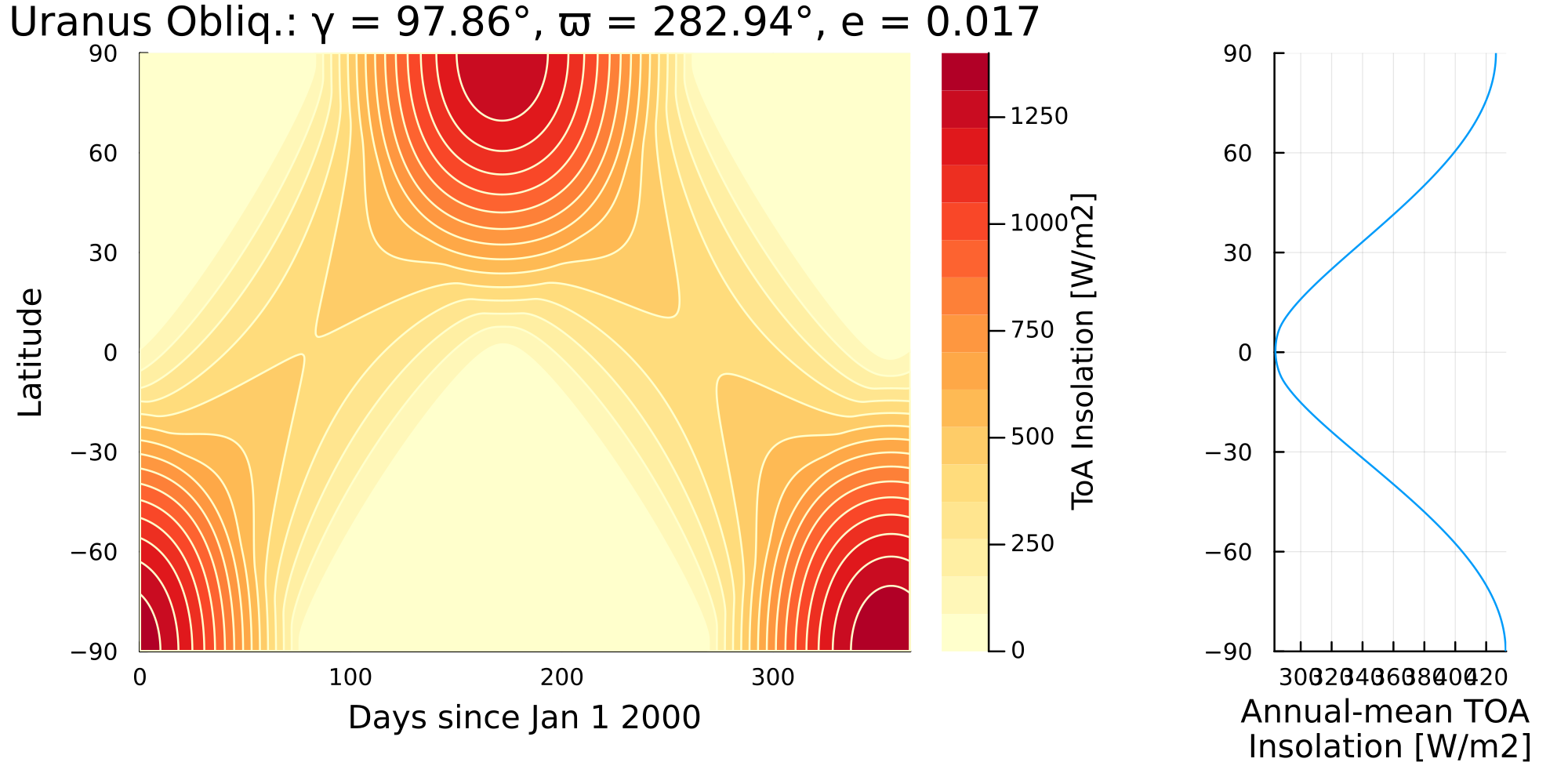
Uranus has an extreme axial tilt of 97.86°, essentially rotating "on its side." Adopting that obliquity while leaving every other parameter at its Earth value isolates the effect of the tilt; it is not a model of Uranus itself, whose year is 84 Earth years and which receives about 1/370 of Earth's solar flux.
# Set obliquity to 97.86° (Uranus's axial tilt)
param_set_uranus = IP.InsolationParameters(FT, (;obliq_epoch = deg2rad(97.86)))
γ4 = IP.obliq_epoch(param_set_uranus)
days, lats, F5 = calc_day_lat_insolation(od, 365, 180, param_set_uranus)

plot_day_lat_insolation(days,lats,F5,"YlOrRd", title, "insol_example3a.png")
plot_day_lat_insolation(days, lats, F5-F0, "PRGn", title, "insol_example3b.png")
Absolute Insolation (top): With extreme obliquity, the insolation pattern is dramatically different:
- Polar regions receive intense summer insolation, far exceeding tropical values, because the summer pole faces almost directly at the sun
- Equatorial regions have two insolation peaks per year, at the equinoxes, when the subsolar point crosses the equator
- Extreme seasons, with polar day and polar night extending over almost the whole planet; note that the subsolar point reaches only 82.1° latitude, since $\sin\delta = \sin\gamma \sin L_s$ and $\sin 97.86° = \sin 82.14°$
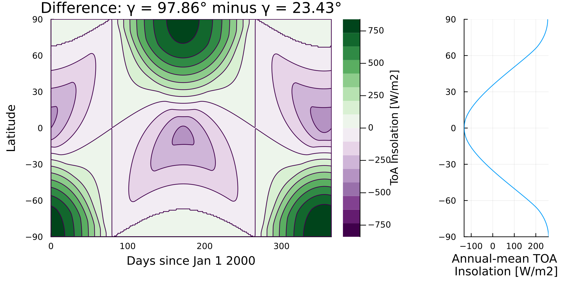
Difference Plot (bottom): Compared to Earth's current configuration:
- Polar summers receive much more insolation, over 750 W/m² more at the summer pole
- The annual mean is inverted: it is now largest at the poles and smallest at the equator. For a near-circular orbit that inversion sets in once the obliquity exceeds about 54°
This extreme case illustrates how orbital parameters fundamentally shape a planet's climate. Such configurations help us understand exotic exoplanets and the range of possible planetary climates.
Summary
These examples demonstrate that Insolation.jl can:
- Calculate diurnal cycles for any location and date
- Visualize latitudinal and seasonal patterns
- Explore sensitivity to orbital parameters
- Model both Earth-like and exotic planetary configurations
For paleoclimate applications with time-varying orbital parameters, see Milankovitch Cycles.