Staggered grid

Velocities $u$, $v$, and $w$ are defined on the faces of the cells, which are coincident with three orthogonal coordinate axes (the Cartesian axes in the case of Oceananigans). Pressure $p$ and tracers $c$ are stored at the cell centers as cell averages. See schematic below of the different control volumes. Other quantities may be defined at other locations. For example, vorticity $\boldsymbol{\omega} = \boldsymbol{\nabla} \times \boldsymbol{v}$ is defined at the cell edges.^[1]

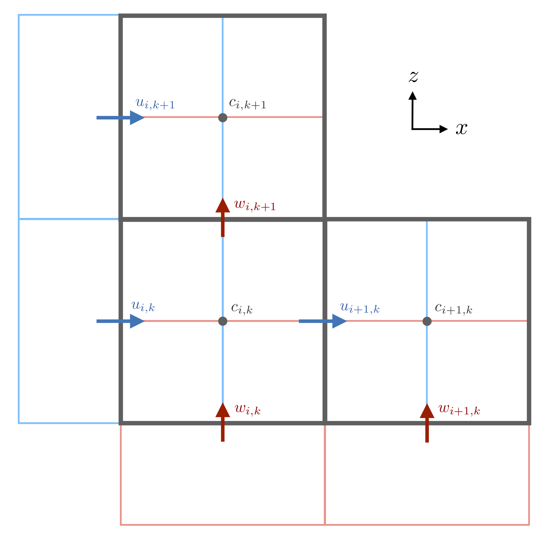A schematic of Oceananigans.jl finite volumes for a two-dimensional staggered grid in $(x, z)$. Tracers $c$ and pressure $p$ are defined at the center of the control volume. The $u$ control volumes are centered on the left and right edges of the pressure control volume while the $w$ control volumes are centered on the top and bottom edges of the pressure control volumes. The indexing convention places the $i^{\rm{th}}$ $u$-node on cell $x$-faces to the left of the $i$ tracer point at cell centers.

This staggered arrangement of variables is more complicated than the collocated grid arrangement but is greatly beneficial as it avoids the odd-even decoupling between the pressure and velocity if they are stored at the same positions. §6.1 of Patankar (1980) discusses this problem in the presence of a zigzag pressure field: on a 1D collocated grid the velocity at the point $i$ is influenced by the pressure at points $i-1$ and $i+1$, and a zigzag pressure field will be felt as a uniform pressure, which is obviously wrong and would reduce the accuracy of the solution. The pressure is effectively taken from a coarser grid than what is actually used. The basic problem is that the momentum equations will use the pressure difference between two alternate points when it should be using two adjacent points.

From the viewpoint of linear algebra, these spurious pressure modes correspond to solutions in the null space of the pressure projection operator with eigenvalue zero and are thus indistinguishable from a uniform pressure field (Sani et al., 1981).

The staggered grid was first introduced by Harlow and Welch (1965) with their marker and cell method. In meteorology and oceanography, this particular staggered grid configuration is referred to as the Arakawa C-grid after Arakawa and Lamb (1977), who investigated four different staggered grids and the unstaggered A-grid for use in an atmospheric model.

Arakawa and Lamb (1977) investigated the dispersion relation of inertia-gravity waves^[2] traveling in the $x$-direction

\[ \omega^2 = f^2 + gHk^2 \, ,\]

in the linearized rotating shallow-water equations for five grids. Here $\omega$ is the angular frequency, $H$ is the height of the fluid and $k$ is the wavenumber in the $x$-direction. Looking at the effect of spatial discretization error on the frequency of these waves they find that the B and C-grids reproduce the dispersion relation most closely out of the five Arakawa and Lamb (1977) (Figure 5). In particular, the dispersion relation for the C-grid is given by

\[ \omega^2 = f^2 \left[ \cos^2 \left( \frac{k\Delta}{2} \right) + 4 \left( \frac{\lambda}{\Delta} \right)^2 \sin^2 \left( \frac{k\Delta}{2} \right) \right] \, ,\]

where $\lambda$ is the wavelength and $\Delta$ is the grid spacing. Paraphrasing p. 184 of Arakawa and Lamb (1977): The wavelength of the shortest resolvable wave is $2\Delta$ with corresponding wavenumber $k = \pi/\Delta$ so it is sufficient to evaluate the dispersion relation over the range $0 < k \Delta < \pi$. The frequency is monotonically increasing for $\lambda / \Delta > \frac{1}{2}$ and monotonically decreasing for $\lambda / \Delta < \frac{1}{2}$. For the fourth smallest wave $\lambda / \Delta = \frac{1}{2}$ we get $\omega^2 = f^2$ which matches the $k = 0$ wave. Furthermore, the group velocity is zero for all $k$. On the other grids, waves with $k \Delta = \pi$ can behave like pure inertial oscillations or stationary waves, which is bad.

The B and C-grids are less oscillatory than the others and quite faithfully simulate geostrophic adjustment. However, the C-grid is the only one that faithfully reproduces the two-dimensional dispersion relation $\omega^2(k, \ell)$, all the other grids have false maxima, and so Arakawa and Lamb (1977) conclude that the C-grid is best for simulating geostrophic adjustment except for abnormal situations in which $\lambda / \Delta$ is less than or close to 1. This seems to have held true for most atmospheric and oceanographic simulations as the C-grid is popular and widely used.