Grids
Oceananigans simulates the dynamics of ocean-flavored fluids by solving equations that conserve momentum, mass, and energy on a grid of finite volumes or "cells". The first decision we make when setting up a simulation is: on what grid are we going to run our simulation? The "grid" captures the
The geometry of the physical domain;
The way that domain is divided into a mesh of finite volumes;
The machine architecture (CPU, GPU, lots of CPUs or lots of GPUs); and
The precision of floating point numbers (double precision or single precision).
We start by making a simple grid that divides a three-dimensional rectangular domain – "a box" – into evenly-spaced cells,
using Oceananigans

grid = RectilinearGrid(topology = (Periodic, Periodic, Bounded),
                       size = (16, 8, 4),
                       x = (0, 64),
                       y = (0, 32),
                       z = (0, 8))

# output
16×8×4 RectilinearGrid{Float64, Periodic, Periodic, Bounded} on CPU with 3×3×3 halo
├── Periodic x ∈ [0.0, 64.0) regularly spaced with Δx=4.0
├── Periodic y ∈ [0.0, 32.0) regularly spaced with Δy=4.0
└── Bounded  z ∈ [0.0, 8.0]  regularly spaced with Δz=2.0
This simple grid
Has a domain that's "periodic" in
, but bounded in . Has
16cells inx,8cells iny, and4cells inz. That means there areHas an
xdimension that spans fromx=0, tox=64. Andyspansy=0toy=32, andzspansz=0toz=8.Has cells that are all the same size, dividing the box in 512 that each has dimension
We can inspect the grid using xnodes, ynodes, and znodes to retrieve node positions. The Center() or Face() argument specifies whether to return positions at cell centers or faces. For the Bounded znodes returns
znodes(grid, Center())

# output
1.0:2.0:7.0znodes(grid, Face())
# output
0.0:2.0:8.0For the Periodic
xnodes(grid, Face())

# output
0.0:4.0:60.0
In building our first grid, we did not specify whether it should be constructed on the CPU or GPU. As a result, the grid was constructed by default on the CPU. Next we build a grid on the GPU that's two-dimensional in z-direction,
using CUDA
architecture = GPU()
z_faces = [0, 1, 3, 6, 10]

grid = RectilinearGrid(architecture,
                       topology = (Periodic, Flat, Bounded),
                       size = (10, 4),
                       x = (0, 20),
                       z = z_faces)

# output
10×1×4 RectilinearGrid{Float64, Periodic, Flat, Bounded} on CUDAGPU with 3×0×3 halo
├── Periodic x ∈ [0.0, 20.0) regularly spaced with Δx=2.0
├── Flat y
└── Bounded  z ∈ [0.0, 10.0] variably spaced with min(Δz)=1.0, max(Δz)=4.0
GPU architecture requires a CUDA-, ROC- or Metal-enabled device
Running this example and creating a grid on the GPU requires a device that supports CUDA, ROC, or Metal. In other words, you must have an Nvidia, AMD, or Apple-compatible GPU available. For more information about CUDA, see the CUDA.jl documentation.
The Flat in topology = (Periodic, Flat, Bounded). So nothing varies in y-derivatives are 0. Also, the keyword argument (or "kwarg" for short) that specifies the size has only two elements rather than 3 as in the first example. The stretched cell interfaces specified by z_faces. Because Bounded, the number of vertical cell interfaces required is Nz + 1 = length(z_faces) = 5, where Nz = 4 is the number of cells in the vertical.
The companion functions xspacings, yspacings, and zspacings return the cell widths in each direction and are most informative when the grid spacing varies. To inspect the variable
Δz = zspacings(grid, Center(), Center(), Center())
[CUDA.@allowscalar Δz[1, 1, k] for k in 1:grid.Nz]

# output
4-element Vector{Float64}:
 1.0
 2.0
 3.0
 4.0
The CUDA.@allowscalar above is needed because scalar indexing is by default not allowed for arrays that live on the GPU. (For more discussion on scalar indexing on GPUs see the Simulation tips section.) The 1.0 to 4.0, matching the growing gaps between successive entries in z_faces.
A bit later in this tutorial, we'll give examples that illustrate how to build a grid that's Distributed across multiple CPUs and GPUs.
Grid types: squares, shells, and mountains
The shape of the physical domain determines what grid type should be used:
RectilinearGridcan be fashioned into lines, rectangles and boxes.LatitudeLongitudeGridrepresents sectors of thin spherical shells, with cells bounded by lines of constant latitude and longitude.OrthogonalSphericalShellGridrepresents sectors of thin spherical shells divided with mesh lines that intersect at right angles (thus, orthogonal) but are otherwise arbitrary.
OrthogonalSphericalShellGrids
See the auxiliary module OrthogonalSphericalShellGrids for recipes that implement useful OrthogonalSphericalShellGrids, including the TripolarGrid (Murray, 1996), RotatedLatitudeLongitudeGrid, LambertConformalConicGrid, and ConformalCubedSpherePanelGrid.
A LambertConformalConicGrid is a regional OrthogonalSphericalShellGrid generated from projected x/y coordinates in meters. It stores longitude and latitude at every staggered horizontal location, together with spherical-shell metrics and cell areas, so that models use the same curvilinear-grid machinery as other OrthogonalSphericalShellGrids. The horizontal topology is Bounded by default and Lambert Conformal Conic grids are not intended for global domains. The projection is conformal rather than equal-area, and longitude is singular at the cone apex or pole, so regional domains should normally avoid placing the apex on a grid point.
For example, a midlatitude regional grid can be constructed from a geographic center, projected spacing, and two standard parallels,
using Oceananigans

grid = LambertConformalConicGrid(size = (8, 6, 1),
                                 center = (-105, 40),
                                 spacing = 20e3,
                                 standard_parallels = (30, 60),
                                 z = (-100, 0))

# output
8×6×1 LambertConformalConicGrid{Float64, Bounded, Bounded, Bounded} on CPU with 3×3×1 halo
├── centered at (λ, φ) = (-105.0, 40.0)
├── longitude: Bounded  extent 1.48547 degrees variably spaced with min(Δλ)=0.185194, max(Δλ)=0.185537
├── latitude:  Bounded  extent 1.11223 degrees variably spaced with min(Δφ)=0.185194, max(Δφ)=0.185537
└── z:         Bounded  z ∈ [-100.0, 0.0]      regularly spaced with Δz=100.0
For example, to make a LatitudeLongitudeGrid that wraps around the sphere, extends for 60 degrees latitude on either side of the equator, and has 5 vertical levels down to 1000 meters, we write
architecture = CPU()

grid = LatitudeLongitudeGrid(architecture,
                             size = (180, 10, 5),
                             longitude = (-180, 180),
                             latitude = (-60, 60),
                             z = (-1000, 0))

# output
180×10×5 LatitudeLongitudeGrid{Float64, Periodic, Bounded, Bounded} on CPU with 3×3×3 halo
├── longitude: Periodic λ ∈ [-180.0, 180.0) regularly spaced with Δλ=2.0
├── latitude:  Bounded  φ ∈ [-60.0, 60.0]   regularly spaced with Δφ=12.0
└── z:         Bounded  z ∈ [-1000.0, 0.0]  regularly spaced with Δz=200.0
The main difference between the syntax for LatitudeLongitudeGrid versus that for the RectilinearGrid are the names of the horizontal coordinates: LatitudeLongitudeGrid has longitude and latitude where RectilinearGrid has x and y.
Extrinsic and intrinsic coordinate systems
Every grid is associated with an "extrinsic" coordinate system: RectilinearGrid uses a Cartesian coordinate system (x, y, z), while LatitudeLongitudeGrid and OrthogonalSphericalShellGrid use the geographic coordinates (λ, φ, z), where λ is longitude, φ is latitude, and z is height. Additionally, OrthogonalSphericalShellGrid has an "intrinsic" coordinate system associated with the orientation of its finite volumes (which, in general, are not aligned with geographic coordinates).
To type λ or φ at the REPL, write either \lambda (for λ) or \varphi (for φ) and then press <TAB>.
Inspecting grids with geographical coordinates
We can inspect grids with geographical coordinates (λ, φ, z) using λnodes, φnodes and also λspacings and φspacings.
If topology is not provided for LatitudeLongitudeGrid, then Oceananigans tries infer it: if the longitude spans 360 degrees, the default x-topology is Periodic; if longitude spans less than 360 degrees x-topology is Bounded.
For example,
grid = LatitudeLongitudeGrid(size = (60, 10, 5),
                             longitude = (0, 60),
                             latitude = (-60, 60),
                             z = (-1000, 0))

# output
60×10×5 LatitudeLongitudeGrid{Float64, Bounded, Bounded, Bounded} on CPU with 3×3×3 halo
├── longitude: Bounded  λ ∈ [0.0, 60.0]    regularly spaced with Δλ=1.0
├── latitude:  Bounded  φ ∈ [-60.0, 60.0]  regularly spaced with Δφ=12.0
└── z:         Bounded  z ∈ [-1000.0, 0.0] regularly spaced with Δz=200.0
is Bounded by default, because longitude = (0, 60).
LatitudeLongitudeGrid topologies
It's still possible to use topology = (Periodic, Bounded, Bounded) even if longitude doesn't span 360 degrees. But neither latitude nor z may be Periodic with LatitudeLongitudeGrid.
Bathymetry, topography, and other irregularities
Irregular or "complex" domains are represented with ImmersedBoundaryGrid, which combines one of the above underlying grids with a type of immersed boundary. The immersed boundaries currently supported are:
GridFittedBottom, which fits a one- or two-dimensional bottom height to the underlying grid, so the active part of the domain is above the bottom height.PartialCellBottom, which is similar toGridFittedBottom, except that the height of the bottommost cell is changed to conform to bottom height, limited to prevent the bottom cells from becoming too thin.GridFittedBoundary, which fits a three-dimensional mask to the grid.
To build an ImmersedBoundaryGrid, we start by building one of the three underlying grids, and then embedding a boundary into that underlying grid.
using Oceananigans.Units

grid = RectilinearGrid(topology = (Bounded, Bounded, Bounded),
                       size = (20, 20, 20),
                       x = (-5kilometers, 5kilometers),
                       y = (-5kilometers, 5kilometers),
                       z = (0, 1kilometer))

# Height and width
H = 100meters
W = 1kilometer

mountain(x, y) = H * exp(-(x^2 + y^2) / 2W^2)
mountain_grid = ImmersedBoundaryGrid(grid, GridFittedBottom(mountain))

# output
20×20×20 ImmersedBoundaryGrid{Float64, Bounded, Bounded, Bounded} on CPU with 3×3×3 halo:
├── immersed_boundary: GridFittedBottom(mean(z)=4.5, min(z)=0.0, max(z)=100.0)
├── underlying_grid: 20×20×20 RectilinearGrid{Float64, Bounded, Bounded, Bounded} on CPU with 3×3×3 halo
├── Bounded  x ∈ [-5000.0, 5000.0] regularly spaced with Δx=500.0
├── Bounded  y ∈ [-5000.0, 5000.0] regularly spaced with Δy=500.0
└── Bounded  z ∈ [0.0, 1000.0]     regularly spaced with Δz=50.0
Yep, that's a Gaussian mountain:
using CairoMakie

h = mountain_grid.immersed_boundary.bottom_height

fig = Figure()
ax = Axis(fig[2, 1], xlabel="x (m)", ylabel="y (m)", aspect=1)
hm = heatmap!(ax, h)
Colorbar(fig[1, 1], hm, vertical=false, label="Bottom height (m)")

fig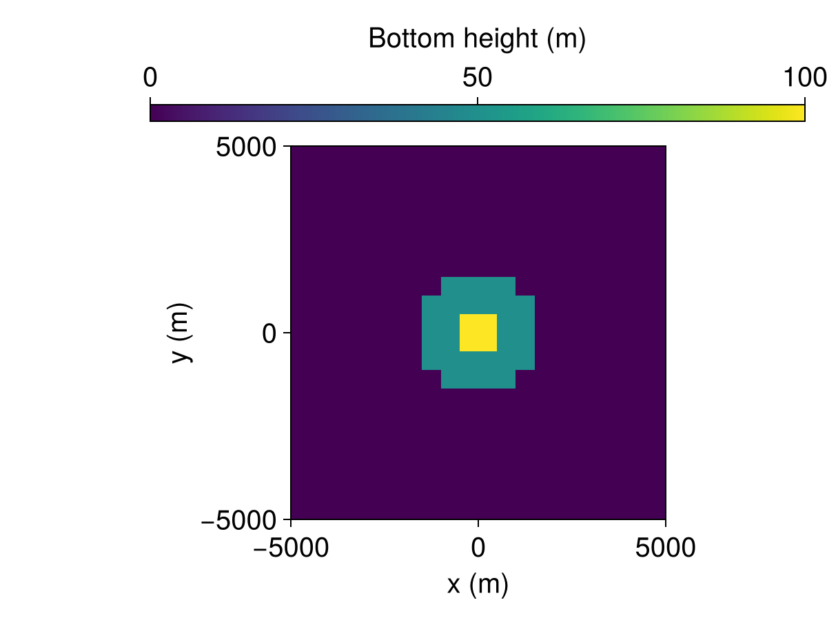
Once more with feeling
In summary, making a grid requires
The machine architecture, or whether data is stored on the CPU, GPU, or distributed across multiple devices or nodes.
Information about the domain geometry. Domains can take a variety of shapes, including
lines (one-dimensional),
rectangles (two-dimensional),
boxes (three-dimensional),
sectors of a thin spherical shells (two- or three-dimensional).
Irregular domains – such as domains that include bathymetry or topography – are represented by using a masking technique to "immerse" an irregular boundary within an "underlying" regular grid. Part of specifying the shape of the domain also requires specifying the nature of each dimension, which may be
Periodic, which means that the dimension circles back onto itself: information leaving the left side of the domain re-enters on the right.Bounded, which means that the two sides of the dimension are either impenetrable (solid walls), or "open", representing a specified external state.Flat, which means nothing can vary in that dimension, reducing the overall dimensionality of the grid.
Defining the number of cells that divide each dimension. The number of cells, with or without explicit specification of the cell interfaces, determines the spatial resolution of the grid.
The representation of floating point numbers, which can be single-precision (
Float32) or double precision (Float64).
Let's dive into each of these options in more detail.
Specifying the machine architecture
The positional argument CPU() or GPU(), specifies the "architecture" of the simulation. By using architecture = GPU(), any fields constructed on grid store their data on an Nvidia GPU, if one is available. By default, the grid will be constructed on the CPU if this argument is omitted. So, for example,
grid     = RectilinearGrid(size=3, z=(0, 1), topology=(Flat, Flat, Bounded))
cpu_grid = RectilinearGrid(CPU(), size=3, z=(0, 1), topology=(Flat, Flat, Bounded))

grid == cpu_grid

# output
true
To use more than one CPU, we use the Distributed architecture,
using Oceananigans

child_architecture = CPU()
architecture = Distributed(child_architecture)
Distributed{CPU} on 1×1×1 across 1 rank:
├── local_rank: 0 of 0-0
├── local_index: [1, 1, 1]
└── connectivity:which allows us to distributed computations across either CPUs or GPUs. In this case, we didn't launch julia on multiple processes using MPI, so we're only "distributed" across 1 process. For more, see Distributed grids.
Specifying the topology for each dimension
The keyword argument topology determines if the grid is one-, two-, or three-dimensional (the current case), and additionally specifies the nature of each dimension. topology is always a Tuple with three elements (a 3-Tuple). For RectilinearGrid, the three elements correspond to Periodic, Bounded, or Flat. A few more examples are,
topology = (Periodic, Periodic, Periodic) # triply periodic
topology = (Periodic, Periodic, Bounded)  # periodic in x, y, bounded in z
topology = (Periodic, Bounded, Bounded)   # periodic in x, but bounded in y, z (a "channel")
topology = (Bounded, Bounded, Bounded)    # bounded in x, y, z (a closed box)
topology = (Periodic, Periodic, Flat)     # two-dimensional, doubly-periodic in x, y (a torus)
topology = (Periodic, Flat, Flat)         # one-dimensional, periodic in x (a line)
topology = (Flat, Flat, Bounded)          # one-dimensional and bounded in z (a single column)
Specifying the size of the grid
The size is a Tuple that specifies the number of grid points in each direction. The number of tuple elements corresponds to the number of dimensions that are not Flat.
The halo size
An additional keyword argument halo allows us to set the number of "halo cells" that surround the core "interior" grid. The default is 3 for each non-flat coordinate. But we can change the halo size, for example,
big_halo_grid = RectilinearGrid(topology = (Periodic, Periodic, Flat),
                                size = (32, 16),
                                halo = (7, 7),
                                x = (0, 2π),
                                y = (0, π))

# output
32×16×1 RectilinearGrid{Float64, Periodic, Periodic, Flat} on CPU with 7×7×0 halo
├── Periodic x ∈ [-6.90805e-17, 6.28319) regularly spaced with Δx=0.19635
├── Periodic y ∈ [-1.07194e-16, 3.14159) regularly spaced with Δy=0.19635
└── Flat z
The halo size has to be set for certain advection schemes that require more halo points than the default 3 in every direction. Note that both size and halo are 2-Tuples, rather than the 3-Tuple that would be required for a three-dimensional grid, or the single number that would be used for a one-dimensional grid.
The dimensions: x, y, z for RectilinearGrid, or latitude, longitude, z for LatitudeLongitudeGrid
These keyword arguments specify the extent and location of the finite volume cells that divide up the three dimensions of the grid. For RectilinearGrid, the dimensions are called x, y, and z, whereas for LatitudeLongitudeGrid the dimensions are called latitude, longitude, and z. The type of each keyword argument determines how the dimension is divided up:
Tuples that specify only the end points indicate that the dimension should be divided into equally-spaced cells. For example,
x = (0, 64)withsize = (16, 8, 4)means that thex-dimension is divided into 16 cells, where the first or leftmost cell interface is located atx = 0and the last or rightmost cell interface is located atx = 64. The width of each cell isΔx=4.0.Vectors and functions alternatively give the location of each cell interface, and thereby may be used to build grids that are divided into cells of varying width.
A complicated example: three-dimensional RectilinearGrid with variable spacing via functions
Next we build a grid that is both Bounded and stretched in both the y and z directions. The purpose of the stretching is to increase grid resolution near the boundaries. We'll do this by using functions to specify the keyword arguments y and z.
Nx = Ny = 64
Nz = 32

Lx = Ly = 1e4
Lz = 1e3

# Note that j varies from 1 to Ny
chebychev_spaced_y_faces(j) = Ly * (1 - cos(π * (j - 1) / Ny)) / 2

# Note that k varies from 1 to Nz
chebychev_spaced_z_faces(k) = - Lz * (1 + cos(π * (k - 1) / Nz)) / 2

grid = RectilinearGrid(size = (Nx, Ny, Nz),
                       topology = (Periodic, Bounded, Bounded),
                       x = (0, Lx),
                       y = chebychev_spaced_y_faces,
                       z = chebychev_spaced_z_faces)

# output
64×64×32 RectilinearGrid{Float64, Periodic, Bounded, Bounded} on CPU with 3×3×3 halo
├── Periodic x ∈ [0.0, 10000.0)  regularly spaced with Δx=156.25
├── Bounded  y ∈ [0.0, 10000.0]  variably spaced with min(Δy)=6.02272, max(Δy)=245.338
└── Bounded  z ∈ [-1000.0, -0.0] variably spaced with min(Δz)=2.40764, max(Δz)=49.0086
We can easily visualize the spacings of ynodes and yspacings to extract the positions and spacings of the nodes from the grid.
yc = ynodes(grid, Center())
zc = znodes(grid, Center())

yf = ynodes(grid, Face())
zf = znodes(grid, Face())

Δy = yspacings(grid, Center())
Δz = zspacings(grid, Center())

using CairoMakie

fig = Figure(size=(1000, 1000))

axy = Axis(fig[1, 1], title="y-grid")
lines!(axy, [0, Ly], [0, 0], color=:gray)
scatter!(axy, yf, 0 * yf, marker=:vline, color=:gray, markersize=25)
scatter!(axy, yc, 0 * yc)
hidedecorations!(axy)
hidespines!(axy)

axΔy = Axis(fig[2, 1]; xlabel = "y (m)", ylabel = "y-spacing (m)")
scatter!(axΔy, yc, Δy)
hidespines!(axΔy, :t, :r)

axz = Axis(fig[3, 1], title="z-grid")
lines!(axz, [-Lz, 0], [0, 0], color=:gray)
scatter!(axz, zf, 0 * zf, marker=:vline, color=:gray, markersize=25)
scatter!(axz, zc, 0 * zc)
hidedecorations!(axz)
hidespines!(axz)

axΔz = Axis(fig[4, 1]; xlabel = "z (m)", ylabel = "z-spacing (m)")
scatter!(axΔz, zc, Δz)
hidespines!(axΔz, :t, :r)

rowsize!(fig.layout, 1, Relative(0.1))
rowsize!(fig.layout, 3, Relative(0.1))

fig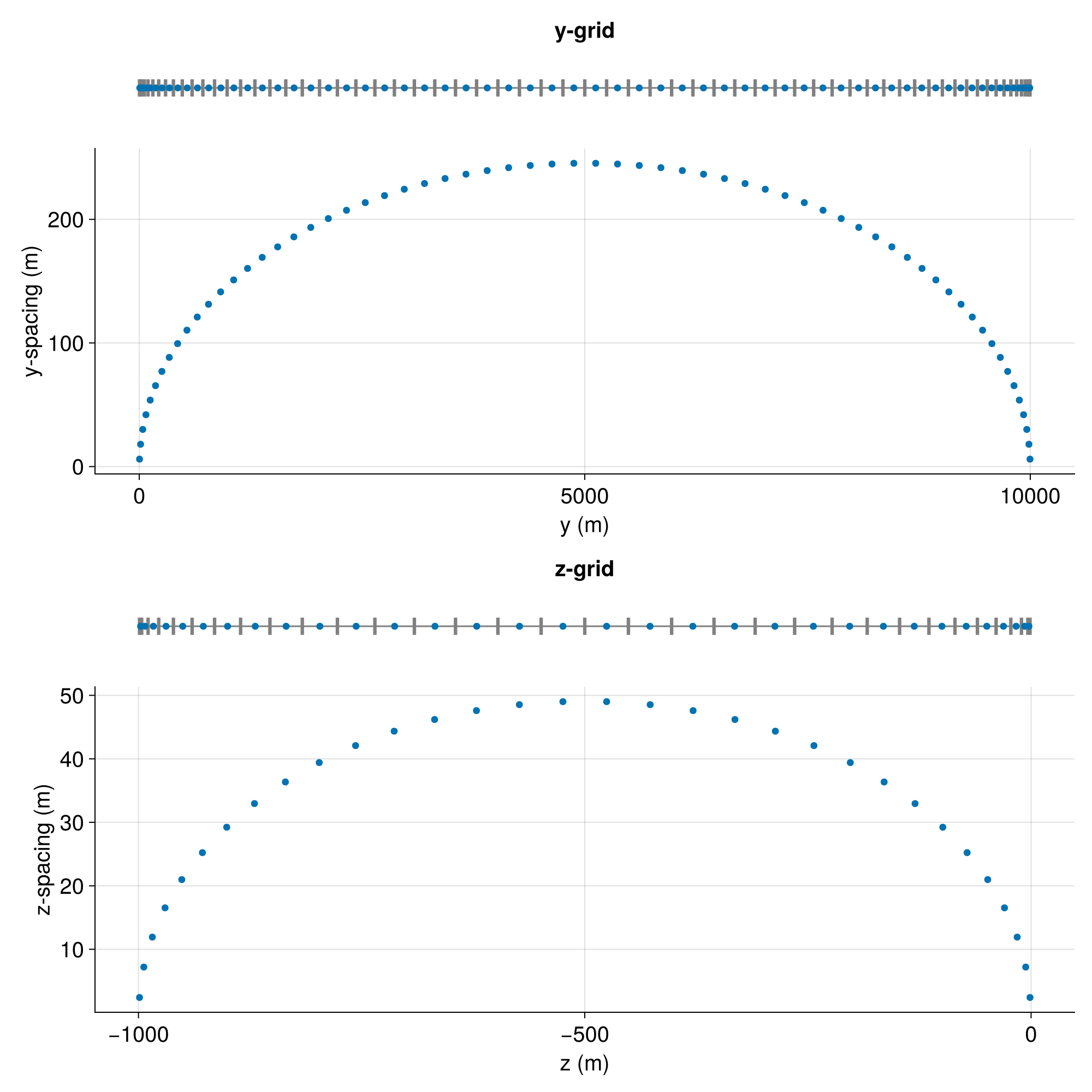
Inspecting LatitudeLongitudeGrid cell spacings
grid = LatitudeLongitudeGrid(size = (1, 44),
                             longitude = (0, 1),
                             latitude = (0, 88),
                             topology = (Bounded, Bounded, Flat))

Δx = xspacings(grid, Center(), Center())

using CairoMakie

fig = Figure()
ax = Axis(fig[1, 1], xlabel="Zonal spacing on 2 degree grid (km)", ylabel="Latitude (degrees)")
scatter!(ax, Δx / 1e3)
fig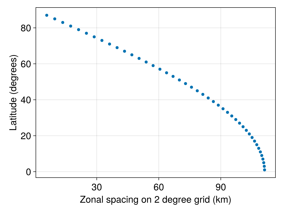
LatitudeLongitudeGrid with variable spacing
The syntax for building a grid with variably-spaced cells is the same as for RectilinearGrid. In our next example, we use a function to build a Mercator grid with a spacing of 2 degrees at the equator,
# Mercator scale factor
scale_factor(φ) = 1 / cosd(φ)

# Compute cell interfaces with Mercator spacing
m = 2 # spacing at the equator in degrees
function latitude_faces(j)
    if j == 1 # equator
        return 0
    else # crudely estimate the location of the jth face
        φ₋ = latitude_faces(j-1)
        φ′ = φ₋ + m * scale_factor(φ₋) / 2
        return φ₋ + m * scale_factor(φ′)
    end
end

Lx = 360
Nx = Int(Lx / m)
Ny = findfirst(latitude_faces.(1:Nx) .> 90) - 2

grid = LatitudeLongitudeGrid(size = (Nx, Ny),
                             longitude = (0, Lx),
                             latitude = latitude_faces,
                             topology = (Bounded, Bounded, Flat))

# output
180×28×1 LatitudeLongitudeGrid{Float64, Bounded, Bounded, Flat} on CPU with 3×3×0 halo
├── longitude: Bounded  λ ∈ [0.0, 360.0]   regularly spaced with Δλ=2.0
├── latitude:  Bounded  φ ∈ [0.0, 77.2679] variably spaced with min(Δφ)=2.0003, max(Δφ)=6.95319
└── z:         Flat z
We've also illustrated the construction of a grid that is Flat in the vertical direction. Now let's plot the metrics for this grid,
φ = φnodes(grid, Center())
Δx = xspacings(grid, Center(), Center())[1, 1:Ny]
Δy = yspacings(grid, Center(), Center())[1, 1:Ny]

using CairoMakie

fig = Figure(size=(800, 400), title="Spacings on a Mercator grid")
axx = Axis(fig[1, 1], xlabel="Zonal spacing (km)", ylabel="Latitude (degrees)")
scatter!(axx, Δx / 1e3, φ)

axy = Axis(fig[1, 2], xlabel="Meridional spacing (km)")
scatter!(axy, Δy / 1e3, φ)

hidespines!(axx, :t, :r)
hidespines!(axy, :t, :l, :r)
hideydecorations!(axy, grid=false)

fig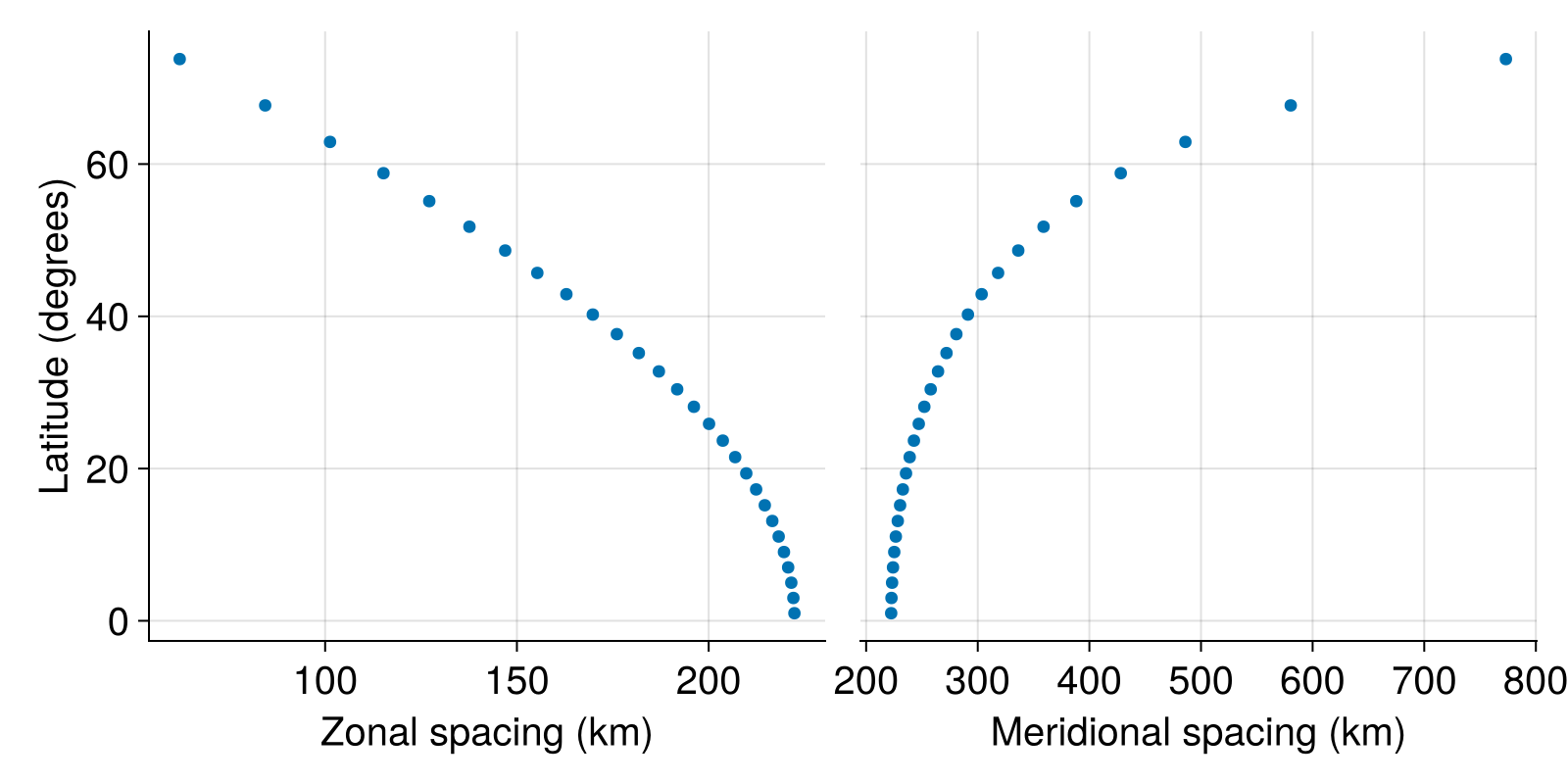
Coordinate helper utilities
As described above, to construct grids with stretched coordinates we need to provide as input either a function the returns the coordinate's interfaces or an array with the interfaces.
Here we showcase some helper utilities that can be used to define few special types of discretizations with variable spacings.
Exponential discretization
ExponentialDiscretization returns a discretization with interfaces that lie on an exponential profile. By that, we mean that a uniformly discretized domain in the range
or
The exponential mappings above have an e-folding controlled by scale
The right-biased map biases the interfaces being closer towards
At the limit
Oceanography-related bias
For vertical coordinates fit for oceanographic purposes, the right-biased mapping is usually more relevant as it implies finer vertical resolution near the ocean's surface.
using Oceananigans.Grids: rightbiased_exponential_mapping, leftbiased_exponential_mapping

using CairoMakie

l, r = 0, 1

ξ  = range(l, stop=r, length=501)
ξp = range(l, stop=r, length=6)   # coarser for plotting

fig = Figure(size=(1200, 550))

axis_labels = (xlabel="uniform ξ / (r - l)",
               ylabel="mapped w / (r - l)")

axl = Axis(fig[1, 1]; title="left-biased map", axis_labels...)
axr = Axis(fig[1, 2]; title="right-biased map", axis_labels...)

for scale in (1/20, 1/5, 1/2, 1e12)
    label = "h / (r-l) = $scale"

    lines!(axl, ξ, leftbiased_exponential_mapping.(ξ, l, r, scale); label)
    scatter!(axl, ξp, leftbiased_exponential_mapping.(ξp, l, r, scale), markersize=20)

    lines!(axr, ξ, rightbiased_exponential_mapping.(ξ, l, r, scale); label)
    scatter!(axr, ξp, rightbiased_exponential_mapping.(ξp, l, r, scale), markersize=20)
end

Legend(fig[2, :], axl, orientation = :horizontal)

fig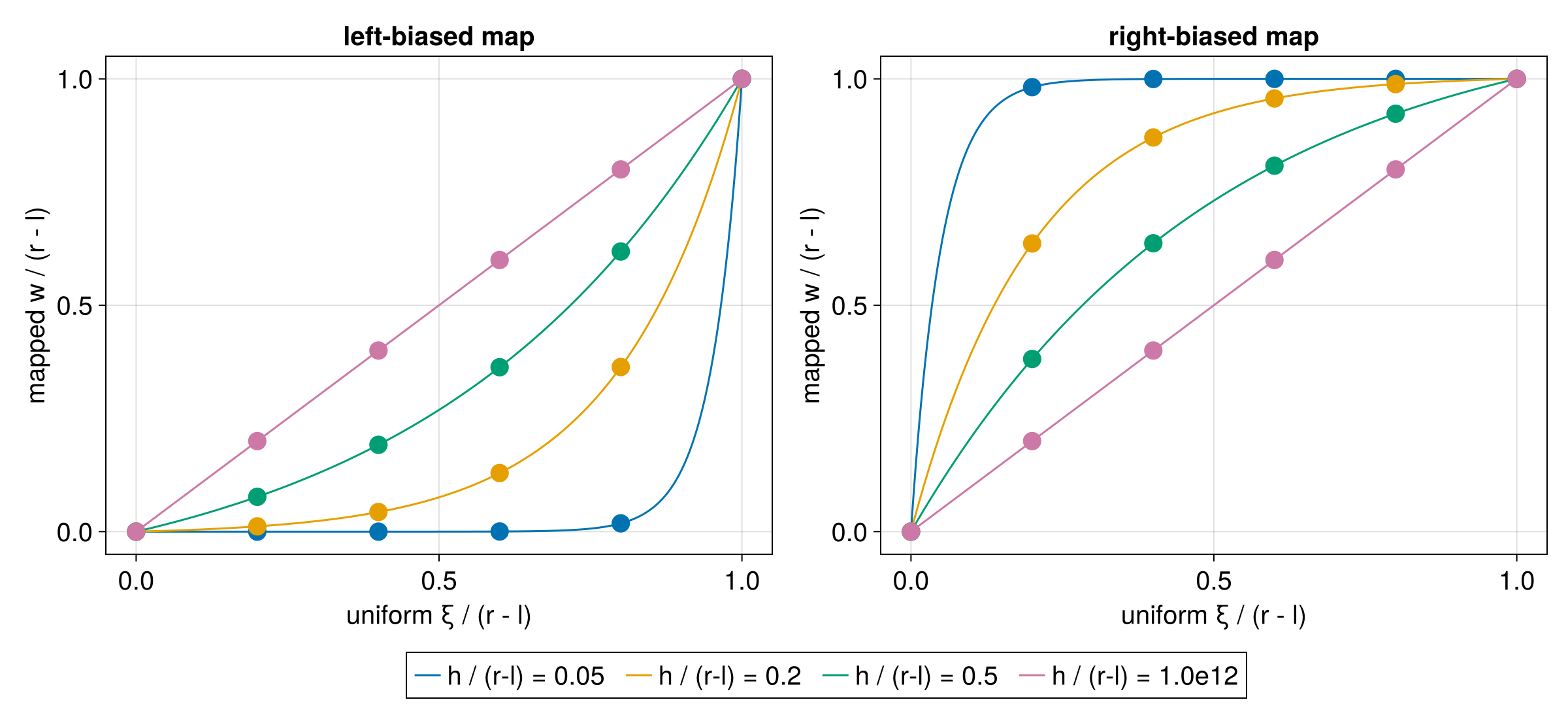
Note that the smallest the ratio
Let's see how we use ExponentialDiscretization. Below we construct a coordinate with 10 cells that spans the range ExponentialDiscretization is right-biased.
using Oceananigans

N = 10
l = -700
r = 300

x = ExponentialDiscretization(N, l, r)
ExponentialDiscretization
├─ size: 10
├─ faces: [-700.0, -303.8614994919127, -63.59135344116919, 82.13985675223907, 170.53030381156742, 224.14181997875644, 256.6588482478361, 276.3814228557754, 288.3437690439604, 295.59929876919114, 300.0]
├─ left: -700.0
├─ right: 300.0
├─ scale: 200.0
└─ bias: :rightNote that above, the default e-folding scale (scale = (r - l) / 5) was used.
We can inspect the interfaces of the coordinate via
[x(i) for i in 1:N+1]11-element Vector{Float64}:
-700.0
-303.8614994919127
-63.59135344116919
82.13985675223907
170.53030381156742
224.14181997875644
256.6588482478361
276.3814228557754
288.3437690439604
295.59929876919114
300.0Being right-biased, note above how the interfaces are closer together near
To demonstrate how the scale
using Oceananigans

N = 10
l = -700
r = 300
extent = r - l

using CairoMakie

fig = Figure(size=(1000, 1000))

scale = extent / 5
x = ExponentialDiscretization(N, l, r; scale)
grid = RectilinearGrid(; size=N, x, topology=(Bounded, Flat, Flat))
xc = xnodes(grid, Center())
xf = xnodes(grid, Face())
Δx = xspacings(grid, Center())

axx1 = Axis(fig[1, 1],  title = "scale = extent / 5")
lines!(axx1, [l, r], [0, 0], color=:gray)
scatter!(axx1, xf, 0 * xf, marker=:vline, color=:gray, markersize=25)
scatter!(axx1, xc, 0 * xc)
axΔx1 = Axis(fig[2, 1]; xlabel = "x (m)", ylabel = "x-spacing (m)")
lΔx = lines!(axΔx1, xf, Δx[1] .+ (xc[1] .- xf) * (extent / scale) / N, color=(:purple, 0.3), linewidth=4)
scatter!(axΔx1, xc, Δx)


scale = extent / 2
x = ExponentialDiscretization(N, l, r; scale)
grid = RectilinearGrid(; size=N, x, topology=(Bounded, Flat, Flat))
xc = xnodes(grid, Center())
xf = xnodes(grid, Face())
Δx = xspacings(grid, Center())

axx2 = Axis(fig[3, 1], title = "scale = extent / 2")
lines!(axx2, [l, r], [0, 0], color=:gray)
scatter!(axx2, xf, 0 * xf, marker=:vline, color=:gray, markersize=25)
scatter!(axx2, xc, 0 * xc)
axΔx2 = Axis(fig[4, 1]; xlabel = "x (m)", ylabel = "x-spacing (m)")
lΔx = lines!(axΔx2, xf, Δx[1] .+ (xc[1] .- xf) * (extent / scale) / N, color=(:purple, 0.3), linewidth=4)
scatter!(axΔx2, xc, Δx)


legend = Legend(fig[5, :], [lΔx], ["slope = (extent / scale) / Nz"], orientation = :horizontal)

for ax in (axx1, axx2)
    hidedecorations!(ax)
    hidespines!(ax)
end

for ax in (axΔx1, axΔx2)
    ylims!(ax, -10, 450)
    hidespines!(ax, :t, :r)
end

rowsize!(fig.layout, 1, Relative(0.1))
rowsize!(fig.layout, 3, Relative(0.1))
fig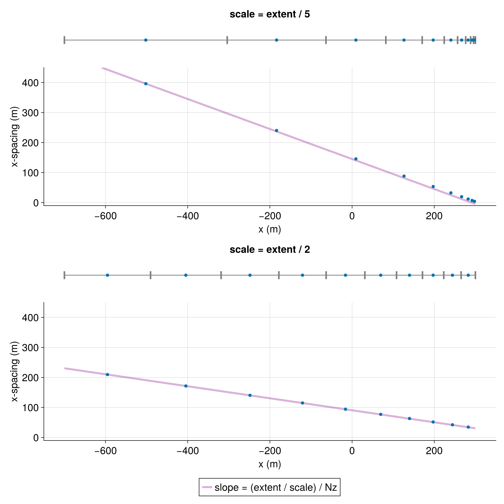
A downside of ExponentialDiscretization discretization is that we don't have tight control on the minimum spacing at the biased edge. To obtain a discretization with a certain minimum spacing we need to play around with the scale
Reference-to-stretched-spacing discretization
ReferenceToStretchedDiscretization returns a discretization with a constant reference spacing over some extent and beyond which the spacing increases with a prescribed stretching law; this allows a tighter control on the spacing at the biased edge. That is, we can prescribe a constant spacing over the top surface_layer_height below which the grid spacing increases following a prescribed stretching law. The downside here is that neither the final discretization extent nor the total number of cells can be prescribed. The discretization's extent is greater or equal from what we prescribe via the keyword argument extent. Also, the total number of cells we end up with depends on the stretching law.
As an example, we build three single-column vertical grids. We use right-biased discretization (i.e., bias = :right) since this way we can have tight control of the spacing at the ocean's surface (bias_edge = 0). The three grids below have constant 30-meter spacing for the top 180 meters. We prescribe to all three a extent = 800 meters and we apply power-law stretching for depths below 120 meters. The bigger the power-law stretching factor is, the further the last interface goes beyond the prescribed depth and/or with less total number of cells.
bias = :right
bias_edge = 0
extent = 800
constant_spacing = 25
constant_spacing_extent = 160

z = ReferenceToStretchedDiscretization(; extent, bias, bias_edge,
                                       constant_spacing,  constant_spacing_extent,
                                       stretching =  PowerLawStretching(1.06))
grid = RectilinearGrid(; size=length(z), z, topology=(Flat, Flat, Bounded))
zf = znodes(grid, Face())
zc = znodes(grid, Center())
Δz = zspacings(grid, Center())
Δz = view(Δz, 1, 1, :)  # for plotting

fig = Figure(size=(800, 550), colgap = 5)

axΔz1 = Axis(fig[1, 1];
             xlabel = "z-spacing (m)",
             ylabel = "z (m)",
             title = "PowerLawStretching(1.06)\n $(length(zf)) cells\n bottom @ z = $(zf[1]) m\n ")

axz1 = Axis(fig[1, 2])

ldepth = hlines!(axΔz1, bias_edge - extent, color = :salmon, linestyle=:dash)
lzbottom = hlines!(axΔz1, zf[1], color = :grey)
scatter!(axΔz1, Δz, zc)
hidespines!(axΔz1, :t, :r)

lines!(axz1, [0, 0], [zf[1], 0], color=:gray)
scatter!(axz1, 0 * zf, zf, marker=:hline, color=:gray, markersize=20)
scatter!(axz1, 0 * zc, zc)
hidedecorations!(axz1)
hidespines!(axz1)


z = ReferenceToStretchedDiscretization(; extent, bias, bias_edge,
                                       constant_spacing,  constant_spacing_extent,
                                       stretching =  PowerLawStretching(1.03))
grid = RectilinearGrid(; size=length(z), z, topology=(Flat, Flat, Bounded))
zf = znodes(grid, Face())
zc = znodes(grid, Center())
Δz = zspacings(grid, Center())
Δz = view(Δz, 1, 1, :)  # for plotting

axΔz2 = Axis(fig[1, 3];
             xlabel = "z-spacing (m)",
             ylabel = "z (m)",
             title = "PowerLawStretching(1.03)\n $(length(zf)) cells\n bottom @ z = $(zf[1]) m\n ")
axz2 = Axis(fig[1, 4])

ldepth = hlines!(axΔz2, bias_edge - extent, color = :salmon, linestyle=:dash)
lzbottom = hlines!(axΔz2, zf[1], color = :grey)
scatter!(axΔz2, Δz, zc)
hidespines!(axΔz2, :t, :r)

lines!(axz2, [0, 0], [zf[1], 0], color=:gray)
scatter!(axz2, 0 * zf, zf, marker=:hline, color=:gray, markersize=20)
scatter!(axz2, 0 * zc, zc)
hidedecorations!(axz2)
hidespines!(axz2)

z = ReferenceToStretchedDiscretization(; extent, bias, bias_edge,
                                       constant_spacing,  constant_spacing_extent,
                                       stretching =  PowerLawStretching(1.03),
                                       maximum_stretching_extent =  500)

grid = RectilinearGrid(; size=length(z), z, topology=(Flat, Flat, Bounded))
zf = znodes(grid, Face())
zc = znodes(grid, Center())
Δz = zspacings(grid, Center())
Δz = view(Δz, 1, 1, :)  # for plotting

axΔz3 = Axis(fig[1, 5];
             xlabel = "z-spacing (m)",
             ylabel = "z (m)",
             title = "PowerLawStretching(1.03)\n $(length(zf)) cells\n bottom @ z = $(zf[1]) m\n maximum_stretching_extent = 500")
axz3 = Axis(fig[1, 6])

ldepth = hlines!(axΔz3, bias_edge - extent, color = :salmon, linestyle=:dash)
lzbottom = hlines!(axΔz3, zf[1], color = :grey)
scatter!(axΔz3, Δz, zc)

hidespines!(axΔz3, :t, :r)

lines!(axz3, [0, 0], [zf[1], 0], color=:gray)
scatter!(axz3, 0 * zf, zf, marker=:hline, color=:gray, markersize=20)
scatter!(axz3, 0 * zc, zc)
hidedecorations!(axz3)
hidespines!(axz3)


linkaxes!(axΔz1, axz1, axΔz2, axz2, axΔz3, axz3)

Legend(fig[2, :], [ldepth, lzbottom], ["prescribed extent", "bottom z interface"], orientation = :horizontal)

colsize!(fig.layout, 2, Relative(0.1))
colsize!(fig.layout, 4, Relative(0.1))
colsize!(fig.layout, 6, Relative(0.1))

fig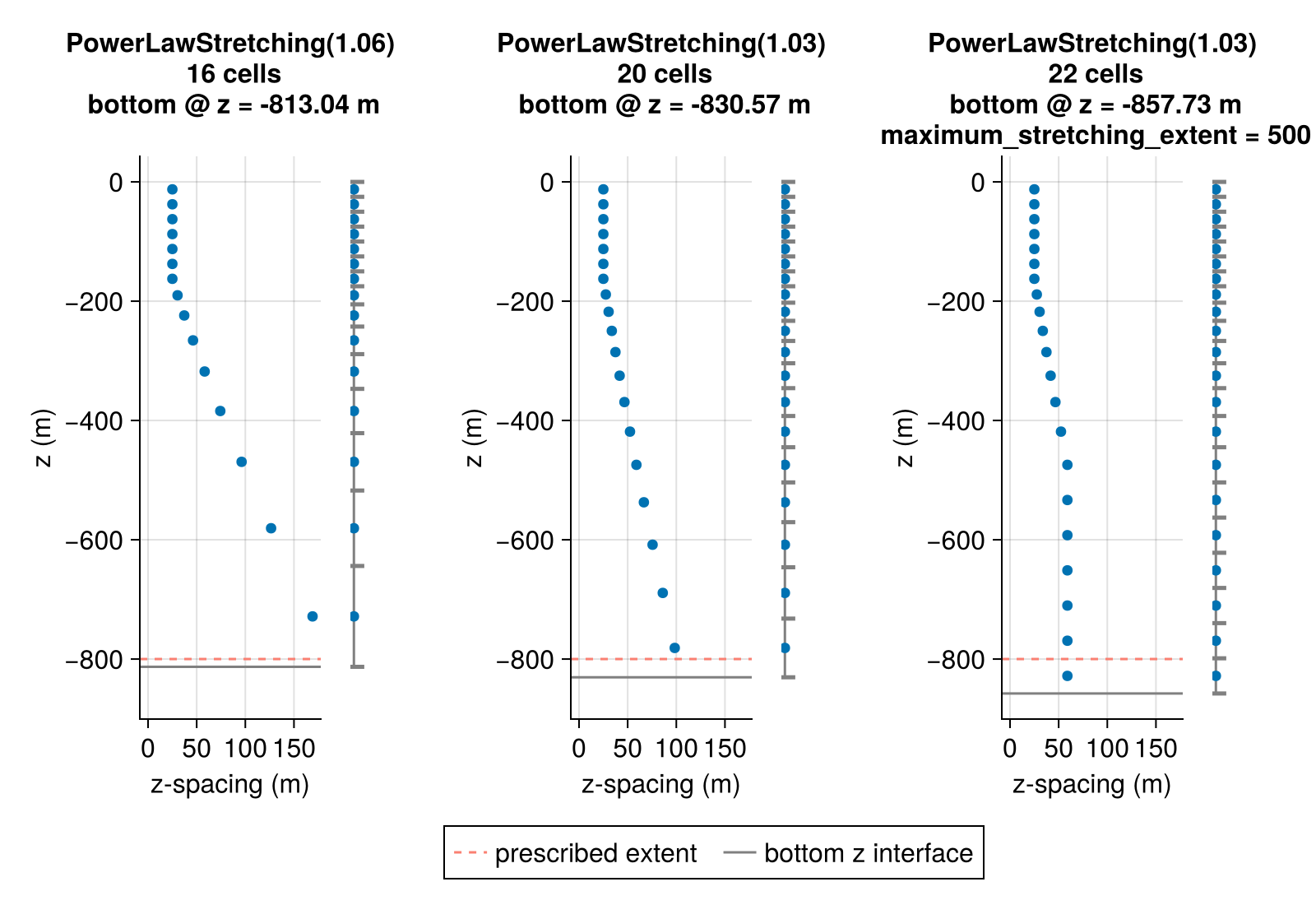
Single-precision grids
To build a grid whose fields are represented with single-precision floating point values, we specify the float_type argument along with the (optional) architecture argument,
architecture = CPU()
float_type = Float32

grid = RectilinearGrid(architecture, float_type,
                       topology = (Periodic, Periodic, Bounded),
                       size = (16, 8, 4),
                       x = (0, 64),
                       y = (0, 32),
                       z = (0, 8))

# output
16×8×4 RectilinearGrid{Float32, Periodic, Periodic, Bounded} on CPU with 3×3×3 halo
├── Periodic x ∈ [0.0, 64.0) regularly spaced with Δx=4.0
├── Periodic y ∈ [0.0, 32.0) regularly spaced with Δy=4.0
└── Bounded  z ∈ [0.0, 8.0]  regularly spaced with Δz=2.0
The same can be accomplished by setting the global default floating point type to Float32:
architecture = CPU()
Oceananigans.defaults.FloatType = Float32

grid = RectilinearGrid(architecture,
                       topology = (Periodic, Periodic, Bounded),
                       size = (16, 8, 4),
                       x = (0, 64),
                       y = (0, 32),
                       z = (0, 8))

# output
16×8×4 RectilinearGrid{Float32, Periodic, Periodic, Bounded} on CPU with 3×3×3 halo
├── Periodic x ∈ [0.0, 64.0) regularly spaced with Δx=4.0
├── Periodic y ∈ [0.0, 32.0) regularly spaced with Δy=4.0
└── Bounded  z ∈ [0.0, 8.0]  regularly spaced with Δz=2.0
Setting the global default is a good approach for building pure Float32 simulations, because this will change all default constructor float types to Float32.
Using single precision
Single precision should be used with care. Users interested in performing single-precision simulations should get in touch via Discussions, and should subject their work to extensive testing and validation.
For more examples see RectilinearGrid and LatitudeLongitudeGrid.
Oceananigans.defaults.FloatType = Float64
nothing

# output
Distributed grids
Note
For the following examples, make sure to have both Oceananigans and MPI in your environment.
Next we turn to the distribution of grids across disparate nodes. This is useful for running simulations that cannot fit on one node. It can also be used to speed up a simulation – provided that the simulation is large enough such that the added cost of communicating information between nodes does not exceed the benefit of dividing up the computation among different nodes.
# Make a simple program that can be written to file
make_distributed_arch = """

using Oceananigans
using Oceananigans.DistributedComputations
using MPI; MPI.Init()
architecture = Distributed()
@onrank 0 @show architecture
@onrank 1 @show architecture
"""

write("distributed_arch_example.jl", make_distributed_arch)

# Run the program from inside julia.
# The program can also be run by exiting julia and running
#
# $ mpiexec -n 2 julia --project distributed_architecture_example.jl
#
# from the terminal.
using MPI
run(`$(mpiexec()) -n 2 $(Base.julia_cmd()) --project distributed_arch_example.jl`)
rm("distributed_arch_example.jl")
architecture = Distributed{CPU} on 2×1×1 across 2 = 2×1×1 ranks:
├── local_rank: 0 of 0-1
├── local_index: [1, 1, 1]
└── connectivity: east=1 west=1
architecture = Distributed{CPU} on 2×1×1 across 2 = 2×1×1 ranks:
├── local_rank: 1 of 0-1
├── local_index: [2, 1, 1]
└── connectivity: east=0 west=0That's what it looks like to build a Distributed architecture. Notice we can choose whether or not to display from a given rank (@onrank 0 @show ....) In this case we choose to display from both ranks, but sometimes it is useful to display only from a single rank, since otherwise ranks can talk over each other making things messy. Also, we used the "default communicator" MPI.COMM_WORLD to determine whether we were on rank 0. This works because Distributed uses communicator = MPI.COMM_WORLD by default (and this should be changed only with great intention). See the Distributed docstring for more information.
Next, let's try to build a distributed grid:
make_distributed_grid = """

using Oceananigans
using Oceananigans.DistributedComputations
using MPI; MPI.Init()

child_architecture = CPU()
architecture = Distributed(child_architecture)

grid = RectilinearGrid(architecture,
                       size = (48, 48, 16),
                       x = (0, 64),
                       y = (0, 64),
                       z = (0, 16),
                       topology = (Periodic, Periodic, Bounded))

@handshake @info grid
"""

write("distributed_grid_example.jl", make_distributed_grid)

using MPI
run(`$(mpiexec()) -n 2 $(Base.julia_cmd()) --project distributed_grid_example.jl`)
┌ Info: 24×48×16 (distributed across 2×1×1 ranks) RectilinearGrid{Float64, FullyConnected, Periodic, Bounded} on Distributed{CPU} on 2×1×1 with 3×3×3 halo
│ ├── FullyConnected x ∈ [0.0, 32.0) regularly spaced with Δx=1.33333
│ ├── Periodic y ∈ [0.0, 64.0) regularly spaced with Δy=1.33333
└ └── Bounded z ∈ [0.0, 16.0] regularly spaced with Δz=1.0
┌ Info: 24×48×16 (distributed across 2×1×1 ranks) RectilinearGrid{Float64, FullyConnected, Periodic, Bounded} on Distributed{CPU} on 2×1×1 with 3×3×3 halo
│ ├── FullyConnected x ∈ [32.0, 64.0) regularly spaced with Δx=1.33333
│ ├── Periodic y ∈ [0.0, 64.0) regularly spaced with Δy=1.33333
└ └── Bounded z ∈ [0.0, 16.0] regularly spaced with Δz=1.0Now we're getting somewhere. Let's note a few things:
For the second example, we explicitly specified
child_architecture = CPU()to distribute the grid across CPUs. Changing this tochild_architecture = GPU()distributes the grid across GPUs.We built the grid with
size = (48, 48, 16), but ended up with a24×48×16grid. Why's that? Well,(48, 48, 16)is the size of the global grid, or in other words, the grid that we would get if we stitched together all the grids from each rank. Here we have two ranks. By default, the local grids are distributed equally inx, which means that each of the two local grids have half of the grids points of the global grid – yielding local sizes of(24, 48, 16).The global grid has topology
(Periodic, Periodic, Bounded), but the local grids have the topology(FullyConnected, Periodic, Bounded). That means that each local grid, which represents half of the global grid and is partitioned inx, is notPeriodicinx. Instead, the west and east sides of each local grid (left and right in thex-direction) are "connected" to another rank.
To drive these points home, let's run the same script, but using 3 processors instead of 2:
run(`$(mpiexec()) -n 3 $(Base.julia_cmd()) --project distributed_grid_example.jl`)┌ Info: 16×48×16 (distributed across 3×1×1 ranks) RectilinearGrid{Float64, FullyConnected, Periodic, Bounded} on Distributed{CPU} on 3×1×1 with 3×3×3 halo
│ ├── FullyConnected x ∈ [0.0, 21.3333) regularly spaced with Δx=1.33333
│ ├── Periodic y ∈ [0.0, 64.0) regularly spaced with Δy=1.33333
└ └── Bounded z ∈ [0.0, 16.0] regularly spaced with Δz=1.0
┌ Info: 16×48×16 (distributed across 3×1×1 ranks) RectilinearGrid{Float64, FullyConnected, Periodic, Bounded} on Distributed{CPU} on 3×1×1 with 3×3×3 halo
│ ├── FullyConnected x ∈ [21.3333, 42.6667) regularly spaced with Δx=1.33333
│ ├── Periodic y ∈ [0.0, 64.0) regularly spaced with Δy=1.33333
└ └── Bounded z ∈ [0.0, 16.0] regularly spaced with Δz=1.0
┌ Info: 16×48×16 (distributed across 3×1×1 ranks) RectilinearGrid{Float64, FullyConnected, Periodic, Bounded} on Distributed{CPU} on 3×1×1 with 3×3×3 halo
│ ├── FullyConnected x ∈ [42.6667, 64.0) regularly spaced with Δx=1.33333
│ ├── Periodic y ∈ [0.0, 64.0) regularly spaced with Δy=1.33333
└ └── Bounded z ∈ [0.0, 16.0] regularly spaced with Δz=1.0Now we have three local grids, each with size (16, 48, 16).
Custom partitions grids in both
To distribute a grid in different ways – for example, in both Partition.
The default Partition is equally distributed in x. To equally distribute in y, we write
make_y_partition = """

using Oceananigans
using Oceananigans.DistributedComputations: Equal
using MPI
MPI.Init()

partition = Partition(y=Equal())

if MPI.Comm_rank(MPI.COMM_WORLD) == 0
    @show partition
end
"""

write("partition_example.jl", make_y_partition)

using MPI
run(`$(mpiexec()) -n 2 $(Base.julia_cmd()) --project partition_example.jl`)
partition = Partition across 2 = 1×2×1 ranks:
└── y: 2Manually specifying ranks in
It's easy to manually configure Partition(x=Rx, y=Ry), where Rx * Ry is the total number of MPI ranks. For example, Partition(x=3, y=2) is compatible with a_program.jl launched via
mpiexec -n 6 julia --project a_program.jlProgrammatically specifying ranks in
Programmatic specification of ranks is often better for applications that need to scale. For this the specification Equal is useful: if the number of ranks in one dimension is specified, and the other is Equal, then the Equal dimension is allocated the remaining workers. For example,
make_xy_partition = """

using Oceananigans
using Oceananigans.DistributedComputations: Equal
using MPI
MPI.Init()

partition = Partition(x=Equal(), y=2)

if MPI.Comm_rank(MPI.COMM_WORLD) == 0
    @show partition
end
"""

write("programmatic_partition_example.jl", make_xy_partition)

using MPI
run(`$(mpiexec()) -n 6 $(Base.julia_cmd()) --project programmatic_partition_example.jl`)
partition = Partition across 6 = 3×2×1 ranks:
├── x: 3
└── y: 2Finally, we can use Equal to partition a grid evenly in
partitioned_grid_example = """

using Oceananigans
using Oceananigans.DistributedComputations: Equal, barrier
using MPI
MPI.Init()

# Total number of ranks
Nr = MPI.Comm_size(MPI.COMM_WORLD)

# Allocate half the ranks to y, and the rest to x
Rx = Nr ÷ 2
partition = Partition(x=Rx, y=Equal())
arch = Distributed(CPU(); partition)

grid = RectilinearGrid(arch,
                       size = (48, 48, 16),
                       x = (0, 64),
                       y = (0, 64),
                       z = (0, 16),
                       topology = (Periodic, Periodic, Bounded))

# Let's see all the grids this time.
for r in 0:Nr-1
    if r == arch.local_rank
        msg = string("On rank ", r, ":", '\n', '\n',
                     arch, '\n',
                     grid)
        @info msg
    end

    barrier(arch)
end
"""

write("equally_partitioned_grids.jl", partitioned_grid_example)

using MPI
run(`$(mpiexec()) -n 4 $(Base.julia_cmd()) --project equally_partitioned_grids.jl`)
┌ Info: On rank 0:
│
│ Distributed{CPU} on 2×2×1 across 4 = 2×2×1 ranks:
│ ├── local_rank: 0 of 0-3
│ ├── local_index: [1, 1, 1]
│ └── connectivity: east=2 west=2 north=1 south=1 southwest=3 southeast=3 northwest=3 northeast=3
│ 24×24×16 (distributed across 2×2×1 ranks) RectilinearGrid{Float64, FullyConnected, FullyConnected, Bounded} on Distributed{CPU} on 2×2×1 with 3×3×3 halo
│ ├── FullyConnected x ∈ [0.0, 32.0) regularly spaced with Δx=1.33333
│ ├── FullyConnected y ∈ [0.0, 32.0) regularly spaced with Δy=1.33333
└ └── Bounded z ∈ [0.0, 16.0] regularly spaced with Δz=1.0
┌ Info: On rank 1:
│
│ Distributed{CPU} on 2×2×1 across 4 = 2×2×1 ranks:
│ ├── local_rank: 1 of 0-3
│ ├── local_index: [1, 2, 1]
│ └── connectivity: east=3 west=3 north=0 south=0 southwest=2 southeast=2 northwest=2 northeast=2
│ 24×24×16 (distributed across 2×2×1 ranks) RectilinearGrid{Float64, FullyConnected, FullyConnected, Bounded} on Distributed{CPU} on 2×2×1 with 3×3×3 halo
│ ├── FullyConnected x ∈ [0.0, 32.0) regularly spaced with Δx=1.33333
│ ├── FullyConnected y ∈ [32.0, 64.0) regularly spaced with Δy=1.33333
└ └── Bounded z ∈ [0.0, 16.0] regularly spaced with Δz=1.0
┌ Info: On rank 2:
│
│ Distributed{CPU} on 2×2×1 across 4 = 2×2×1 ranks:
│ ├── local_rank: 2 of 0-3
│ ├── local_index: [2, 1, 1]
│ └── connectivity: east=0 west=0 north=3 south=3 southwest=1 southeast=1 northwest=1 northeast=1
│ 24×24×16 (distributed across 2×2×1 ranks) RectilinearGrid{Float64, FullyConnected, FullyConnected, Bounded} on Distributed{CPU} on 2×2×1 with 3×3×3 halo
│ ├── FullyConnected x ∈ [32.0, 64.0) regularly spaced with Δx=1.33333
│ ├── FullyConnected y ∈ [0.0, 32.0) regularly spaced with Δy=1.33333
└ └── Bounded z ∈ [0.0, 16.0] regularly spaced with Δz=1.0
┌ Info: On rank 3:
│
│ Distributed{CPU} on 2×2×1 across 4 = 2×2×1 ranks:
│ ├── local_rank: 3 of 0-3
│ ├── local_index: [2, 2, 1]
│ └── connectivity: east=1 west=1 north=2 south=2 southwest=0 southeast=0 northwest=0 northeast=0
│ 24×24×16 (distributed across 2×2×1 ranks) RectilinearGrid{Float64, FullyConnected, FullyConnected, Bounded} on Distributed{CPU} on 2×2×1 with 3×3×3 halo
│ ├── FullyConnected x ∈ [32.0, 64.0) regularly spaced with Δx=1.33333
│ ├── FullyConnected y ∈ [32.0, 64.0) regularly spaced with Δy=1.33333
└ └── Bounded z ∈ [0.0, 16.0] regularly spaced with Δz=1.0