Quick start

This code:

using Oceananigans

grid = RectilinearGrid(size = (128, 128),
                       x = (0, 2π),
                       y = (0, 2π),
                       topology = (Periodic, Periodic, Flat))

model = NonhydrostaticModel(; grid, advection=WENO())

ϵ(x, y) = 2rand() - 1
set!(model, u=ϵ, v=ϵ)

simulation = Simulation(model; Δt=0.01, stop_iteration=100)
run!(simulation)

[ Info: Initializing simulation...
[ Info:     ... simulation initialization complete (2.431 seconds)
[ Info: Executing initial time step...
[ Info:     ... initial time step complete (3.682 seconds).
[ Info: Simulation is stopping after running for 7.236 seconds.
[ Info: Model iteration 100 equals or exceeds stop iteration 100.

runs 100 time steps of a two-dimensional turbulence simulation with 128² finite volume cells and a fifth-order upwinded WENO advection scheme. It's quite similar to the two-dimensional turbulence example.

Visualization

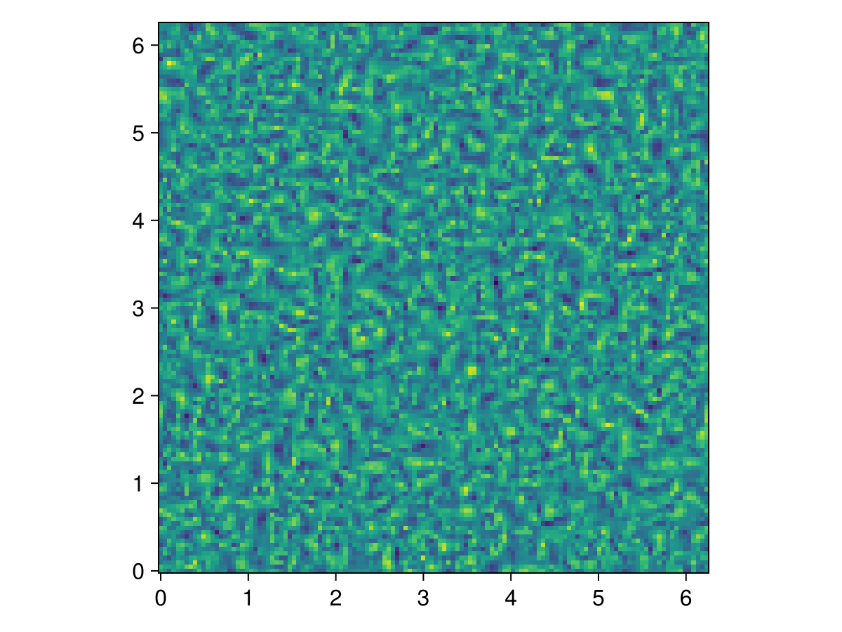
They say that a Makie visualization is worth a thousand Unicode characters, so let's plot vorticity,

using CairoMakie

u, v, w = model.velocities
ζ = Field(∂x(v) - ∂y(u))
compute!(ζ)

heatmap(ζ, axis=(; aspect=1))

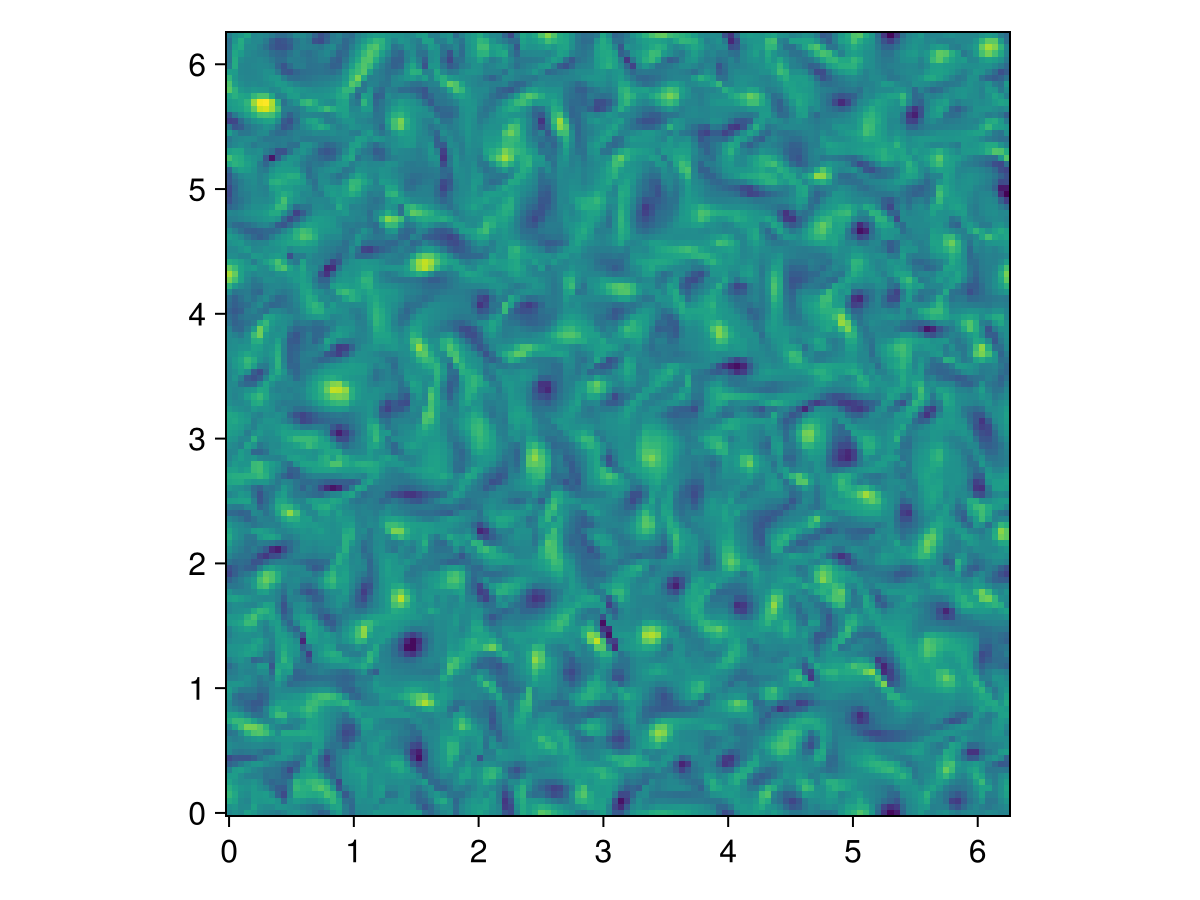
A few more time-steps, and it's starting to get a little diffuse!

simulation.stop_iteration += 400
run!(simulation)

compute!(ζ)
heatmap(ζ, axis=(; aspect=1))

They always cheat with too-simple "quick" starts

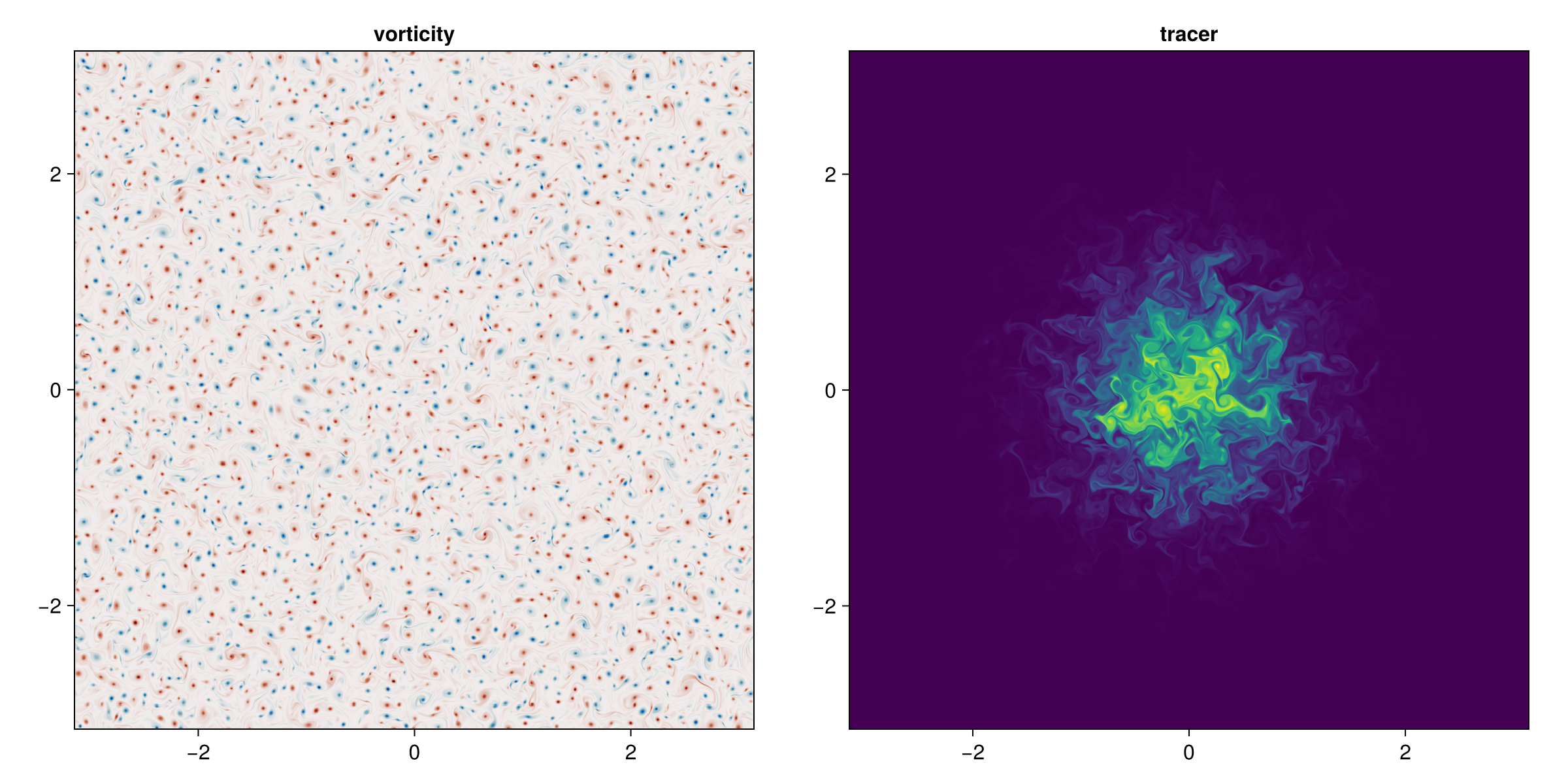
Fine, we'll re-run this code on the GPU. But we're a little greedy, so we'll also crank up the resolution, throw in a TimeStepWizard to update simulation.Δt adaptively, and add a passive tracer initially concentrated in the center of the domain which will make for an even prettier figure of the final state:

using Oceananigans
using CairoMakie

grid = RectilinearGrid(GPU(),
                       size = (1024, 1024),
                       x = (-π, π),
                       y = (-π, π),
                       topology = (Periodic, Periodic, Flat))

model = NonhydrostaticModel(; grid, advection=WENO(), tracers=:c)

δ = 0.5
cᵢ(x, y) = exp(-(x^2 + y^2) / 2δ^2)
ϵ(x, y) = 2rand() - 1
set!(model, u=ϵ, v=ϵ, c=cᵢ)

simulation = Simulation(model; Δt=1e-3, stop_time=10)
conjure_time_step_wizard!(simulation, cfl=0.2, IterationInterval(10))
run!(simulation)

u, v, w = model.velocities
ζ = Field(∂x(v) - ∂y(u))
compute!(ζ)

fig = Figure(size=(1200, 600))
axζ = Axis(fig[1, 1], aspect=1, title="vorticity")
axc = Axis(fig[1, 2], aspect=1, title="tracer")
heatmap!(axζ, ζ, colormap=:balance)
heatmap!(axc, model.tracers.c)
current_figure()

See how we did that? We passed the positional argument GPU() to RectilinearGrid. (This only works if a GPU is available, of course, and CUDA.jl is configured.)

Well, that was tantalizing

But you'll need to know a lot more to become a productive, Oceananigans-wielding computational scientist (spherical grids, forcing, boundary conditions, turbulence closures, output writing, actually labeling your axes... 🤯). It'd be best to move on to the one-dimensional diffusion example.