Universal Functions in SurfaceFluxes.jl

UniversalFunctions.jl provides the stability functions (universal functions) required by Monin-Obukhov Similarity Theory (MOST) to calculate surface fluxes of momentum and heat/tracers. These functions describe the non-dimensional gradients of wind speed and potential temperature/tracers as a function of the stability parameter

\[\zeta = \frac{z - d}{L},\]

where $z$ is the height above surface, $d$ is the displacement height, and $L$ is the Obukhov length.

The module supports three distinct parameterizations:

1. Businger: The classic Businger-Dyer formulations (Businger et al. 1971, Dyer 1974).
2. Gryanik: Improved functions for the stable boundary layer (Gryanik et al. 2020).
3. Grachev: Functions derived from the SHEBA experiment for stable conditions over sea ice (Grachev et al. 2007).

Mathematical Framework

In MOST, the vertical gradients of mean wind speed ($u$) and potential temperature ($\theta$) are scaled by the friction velocity ($u_*$) and temperature scale ($\theta_*$),

\[\begin{equation} \frac{\kappa (z-d)}{u_*} \frac{\partial u}{\partial z} = \phi_m(\zeta) \end{equation}\]

and

\[\begin{equation} \frac{\kappa (z-d)}{\theta_*} \frac{\partial \theta}{\partial z} = \phi_h(\zeta), \end{equation}\]

where $\phi_m$ and $\phi_h$ are the universal stability functions for momentum and heat, respectively, and $\kappa \approx 0.4$ is the von Kármán constant.

Neutral Limits

A key consistency rule in SurfaceFluxes.jl is how the functions behave at neutral stability ($\zeta = 0$):

• Momentum: $\phi_m(0) = 1$.
• Heat/Scalars: $\phi_h(0) = \text{Pr}_0$.
  • For Businger and Gryanik, $\text{Pr}_0$ is a configurable parameter (typically 0.74 or 0.98).
  • For Grachev, the fit of Grachev et al. (2007) has $\phi_h(0) = 1$, so the ClimaParams constructor GrachevParams(toml_dict) sets Pr_0 = 1 (overriding prandtl_number_0_grachev); the keyword constructor accepts any value. The variable is retained in the equations for structural consistency.

Integrated Stability Correction Functions

We also define the integrated stability correction functions ($\psi$) that define corrections to logarithmic profiles, including their layer-averaged forms ($\Psi$) used with finite-volume schemes:

• The function $\psi(\zeta)$: The standard integral form used to correct point profiles (for finite-difference schemes):

\[\begin{equation} \psi(\zeta) = \int_{0}^{\zeta} \frac{\phi(0) - \phi(x)}{x} dx. \end{equation}\]

This function is used to obtain the wind profile:

\[\begin{equation} u(z) = \frac{u_*}{\kappa} \left[ \ln\left(\frac{z-d}{z_{0m}}\right) - \psi_m(\zeta) + \psi_m(\zeta_{0m}) \right], \end{equation}\]

where $\zeta_{0m} = z_{0m}/L$ is the stability parameter at the roughness height $z_{0m}$.

Similarly, the potential temperature profile is obtained using the heat stability correction function:

\[\begin{equation} \theta(z) = \theta_0 + \frac{\theta_*}{\kappa} \left[ \phi_h(0) \ln\left(\frac{z-d}{z_{0h}}\right) - \psi_h(\zeta) + \psi_h(\zeta_{0h}) \right], \end{equation}\]

where $\theta_0$ is the surface potential temperature, $\zeta_{0h} = z_{0h}/L$ is the stability parameter at the roughness height $z_{0h}$, and $\theta_*$ is the temperature scale. The bracketed terms are the dimensionless profiles $F_m$ and $F_h$ that enter the bulk Richardson number $Ri_b(\zeta)$ and the exchange coefficients; with a roughness-sublayer correction, they become $\widehat{F} = F + P$ (see Surface Fluxes Theory).

• The function $\Psi(\zeta)$: The layer-averaged form required when model variables represent cell averages (in finite-volume schemes) rather than point values (Nishizawa & Kitamura, 2018):

\[\begin{equation} \Psi(\zeta) = \frac{1}{\zeta} \int_{0}^{\zeta} \psi(x) dx. \end{equation}\]

For finite-volume schemes, where fluxes are computed using cell-averaged values, this function is used to obtain the vertical profiles. For example, the layer-averaged wind speed is calculated as:

\[\begin{equation} \bar{u}(z) = \frac{u_*}{\kappa} \left[ \ln\left(\frac{z-d}{z_{0m}}\right) - \Psi_m(\zeta) + \frac{z_{0m}}{\Delta z} \Psi_m(\zeta_{0m}) + \left(1 - \frac{z_{0m}}{\Delta z}\right)(\psi_m(\zeta_{0m}) - 1) \right] \end{equation}\]

where $\Delta z = z - d$ is the thickness of the first layer, and the profile is the average $(1/\Delta z)\int_{z_{0m}}^{\Delta z}$ of the point profile. For heat and scalars, the logarithm and the $-1$ are multiplied by the neutral slope $\phi_h(0) = \text{Pr}_0$, so that the last term is $(1 - z_{0h}/\Delta z)(\psi_h(\zeta_{0h}) - \text{Pr}_0)$.

1. Businger-Dyer Functions

The Businger parameterization is the standard formulation for the unstable and weakly stable boundary layer. Our implementation follows the forms detailed in Nishizawa & Kitamura (2018), which provides a unified treatment of both stable and unstable conditions.

Parameter Structure

The BusingerParams struct contains:

• Pr_0: The neutral Prandtl number
• a_m, a_h: Linear coefficients for stable conditions (denoted as $\beta$ in some texts)
• b_m, b_h: Coefficients inside the unstable sqrt/cbrt terms (denoted as $\gamma$ in the unstable forms)

Unstable Conditions ($\zeta < 0$)

For unstable conditions, the functions follow the Dyer-Hicks form (Nishizawa & Kitamura 2018, Eqs. A1-A2 for $L < 0$), scaled by $\text{Pr}_0$ for heat to ensure continuity at $\zeta=0$:

\[\begin{equation} \phi_m(\zeta) = (1 - b_m \zeta)^{-1/4}, \end{equation}\]

and

\[\begin{equation} \phi_h(\zeta) = \text{Pr}_0 (1 - b_h \zeta)^{-1/2}, \end{equation}\]

where, typically, $b_m=15$ and $b_h=9$. These defaults are the values of Businger et al. (1971), which were derived with $\kappa = 0.35$; Högström (1988) re-evaluated the constants for $\kappa = 0.4$.

The corresponding integrated functions ($\psi$) involve logarithmic and arctangent terms (Nishizawa & Kitamura 2018, Eqs. A3-A4 for $L < 0$):

\[\begin{equation} \psi_m(\zeta) = \ln\left[\frac{(1 + x)^2(1 + x^2)}{8}\right] - 2\tan^{-1}(x) + \frac{\pi}{2}, \end{equation}\]

where $x = (1 - b_m \zeta)^{1/4}$. For heat, the function is scaled by $\text{Pr}_0$:

\[\begin{equation} \psi_h(\zeta) = 2 \text{Pr}_0 \ln\left(\frac{1 + y}{2}\right), \end{equation}\]

where $y = (1 - b_h \zeta)^{1/2}$.

Stable Conditions ($\zeta \ge 0$)

For stable conditions, the Businger-Dyer functions are linear:

\[\begin{equation} \phi_m(\zeta) = 1 + a_m \zeta \end{equation}\]

and

\[\begin{equation} \phi_h(\zeta) = \text{Pr}_0 + a_h \zeta. \end{equation}\]

The integrated forms are (Nishizawa & Kitamura 2018, Eqs. A3-A4 for $L \ge 0$):

\[\begin{equation} \psi_m(\zeta) = -a_m \zeta \end{equation}\]

and

\[\begin{equation} \psi_h(\zeta) = -a_h \zeta, \end{equation}\]

Because the stable heat function is $\phi_h = \text{Pr}_0 + a_h \zeta$ (Businger et al. 1971), $\text{Pr}_0$ enters only through the neutral slope $\phi_h(0)$; $\psi_h$ and $\Psi_h$ for $\zeta \ge 0$ carry no factor $\text{Pr}_0$.

Layer-Averaged Forms

The layer-averaged functions $\Psi$ are implemented for both momentum and heat transport, following Nishizawa & Kitamura (2018, Eqs. A5-A6, A13-A14), with the unstable heat functions scaled by $\text{Pr}_0$.

Stable Conditions ($\zeta \ge 0$):

For stable conditions, the layer-averaged functions reduce to:

\[\begin{equation} \Psi_m(\zeta) = -\frac{a_m \zeta}{2} \end{equation}\]

and

\[\begin{equation} \Psi_h(\zeta) = -\frac{a_h \zeta}{2}. \end{equation}\]

Unstable Conditions ($\zeta < 0$):

For unstable conditions, computations follow Nishizawa & Kitamura (2018, Eqs. A5-A6), with appropriate $\text{Pr}_0$ scaling for heat.

For momentum:

\[\begin{equation} \Psi_m(\zeta) = \ln\left[\frac{(1 + x)^2(1 + x^2)}{8}\right] - 2\tan^{-1}(x) + \frac{\pi}{2} - 1 + \frac{1 - x^3}{3b_m \zeta/4}, \end{equation}\]

where $x = (1 - b_m \zeta)^{1/4}$. For small $\zeta$, this reduces to $\Psi_m(\zeta) \approx -b_m \zeta/8$ (Nishizawa & Kitamura 2018, Eq. A13). The code uses the linear limit only for $|\zeta|$ below machine epsilon, to avoid division by zero; elsewhere, expm1 and log1p limit cancellation.

For heat:

\[\begin{equation} \Psi_h(\zeta) = \text{Pr}_0 \left[ 2\ln\left(\frac{1 + y}{2}\right) + \frac{2(1 - y)}{b_h \zeta} - 1 \right], \end{equation}\]

where $y = (1 - b_h \zeta)^{1/2}$. For small $\zeta$, this reduces to $\Psi_h(\zeta) \approx - \text{Pr}_0 b_h \zeta/4$ (Nishizawa & Kitamura 2018, Eq. A14, with the scaling by $\text{Pr}_0$ applied).

2. Gryanik Universal Functions

The Gryanik et al. (2020) parameterization is designed to improve surface flux calculations in the stable boundary layer. It addresses issues where standard functions underestimate fluxes in very stable conditions.

Parameter Structure

The GryanikParams struct contains:

• Pr_0: Neutral Prandtl number (Gryanik et al. recommend $\text{Pr}_0 \approx 0.98$)
• a_m, b_m: Coefficients for momentum stability function
• a_h, b_h: Coefficients for heat stability function
• b_m_unstable, b_h_unstable: Parameters for unstable branch (automatically set to Businger values)

Stable Conditions ($\zeta > 0$)

Gryanik proposes new forms that remain valid across a wide stability range.

Momentum ($\phi_m$):

\[\begin{equation} \phi_m(\zeta) = 1 + \frac{a_m \zeta}{(1 + b_m \zeta)^{2/3}}. \end{equation}\]

Heat ($\phi_h$):

\[\begin{equation} \phi_h(\zeta) = \text{Pr}_0 \left( 1 + \frac{a_h \zeta}{1 + b_h \zeta} \right). \end{equation}\]

Note that $\phi_h(0) = \text{Pr}_0$ for Gryanik, consistent with our Businger implementation.

Integrated Corrections ($\psi$): The code implements the analytical integrals derived in the paper:

\[\begin{equation} \psi_m(\zeta) = -3 \frac{a_m}{b_m} \left[ (1 + b_m \zeta)^{1/3} - 1 \right], \end{equation}\]

and

\[\begin{equation} \psi_h(\zeta) = -\text{Pr}_0 \frac{a_h}{b_h} \ln(1 + b_h \zeta). \end{equation}\]

Layer-Averaged Forms ($\Psi$): The layer-averaged functions are analytically derived from the $\psi$ functions:

\[\begin{equation} \Psi_m(\zeta) = 3\frac{a_m}{b_m} - \frac{9 a_m}{4 b_m^2 \zeta} \left[ (1 + b_m \zeta)^{4/3} - 1 \right] \end{equation}\]

and

\[\begin{equation} \Psi_h(\zeta) = -\frac{\text{Pr}_0 a_h}{b_h \zeta} \left[ \left(\frac{1}{b_h} + \zeta\right) \ln(1 + b_h \zeta) - \zeta \right]. \end{equation}\]

Unstable Conditions ($\zeta < 0$)

Gryanik et al. (2020) address only stable stratification. For the unstable regime, our implementation uses the Businger unstable forms with coefficients b_m_unstable and b_h_unstable (which are set to the Businger parameters). The unstable heat function is scaled by $\text{Pr}_0$ to ensure a continuous transition at the neutral limit ($\zeta=0$):

\[\begin{equation} \phi_h(\zeta) = \text{Pr}_0 (1 - b_{h,\text{unstable}} \zeta)^{-1/2} \end{equation}\]

3. Grachev Universal Functions

The Grachev et al. (2007) functions were derived from measurements of the stable atmospheric boundary layer over sea ice from the SHEBA dataset.

Parameter Structure

The GrachevParams struct contains:

• Pr_0: Neutral Prandtl number (explicitly set to 1.0)
• a_m, b_m: Coefficients for momentum stability function
• a_h, b_h, c_h: Coefficients for heat stability function (note: c_h is the coefficient for the linear $\zeta$ term in the denominator)
• b_m_unstable, b_h_unstable: Parameters for unstable branch (automatically set to the Businger parameters)

Stable Conditions ($\zeta > 0$)

Momentum ($\phi_m$):

\[\begin{equation} \phi_m(\zeta) = 1 + \frac{a_m \zeta (1 + \zeta)^{1/3}}{1 + b_m \zeta}. \end{equation}\]

Heat ($\phi_h$):

\[\begin{equation} \phi_h(\zeta) = \text{Pr}_0 \left( 1 + \frac{a_h \zeta + b_h \zeta^2}{1 + c_h \zeta + \zeta^2} \right). \end{equation}\]

Integrated Corrections ($\psi$): The integrated forms are complex, involving multiple logarithmic and arctangent terms. See Grachev et al. (2007, Eqs. 12 and 13) for the full derivation.

For momentum (Grachev et al. 2007, Eq. 12):

\[\begin{equation} \psi_m(\zeta) = -3\frac{a_m}{b_m}(x - 1) + \frac{a_m B_m}{2 b_m} \left[ 2\ln\left(\frac{x + B_m}{1 + B_m}\right) - \ln\left(\frac{x^2 - x B_m + B_m^2}{1 - B_m + B_m^2}\right) + 2\sqrt{3}\left(\arctan\left(\frac{2x - B_m}{\sqrt{3} B_m}\right) - \arctan\left(\frac{2 - B_m}{\sqrt{3} B_m}\right)\right) \right], \end{equation}\]

where $x = (1 + \zeta)^{1/3}$ and $B_m = ((1 - b_m)/b_m)^{1/3}$.

For heat (Grachev et al. 2007, Eq. 13):

\[\begin{equation} \psi_h(\zeta) = \text{Pr}_0 \left( -\frac{b_h}{2} \ln(1 + c_h \zeta + \zeta^2) + \left[-\frac{a_h}{B_h} + \frac{b_h c_h}{2 B_h}\right] \left[\ln\left(\frac{2\zeta + c_h - B_h}{2\zeta + c_h + B_h}\right) - \ln\left(\frac{c_h - B_h}{c_h + B_h}\right)\right] \right), \end{equation}\]

where $B_h = \sqrt{c_h^2 - 4}$. The code multiplies the entire result by $\text{Pr}_0$, which the ClimaParams constructor sets to 1 for this parameterization.

Unstable Conditions ($\zeta < 0$)

As for the Gryanik parameterization, the Grachev parameterization falls back to the Businger-Dyer forms for unstable conditions, using the b_m_unstable and b_h_unstable parameters. The unstable heat function is scaled by the parameterization's own $\text{Pr}_0$, so $\phi_h$ is continuous at $\zeta = 0$.

Visualization of Universal Functions

The following plots compare the behavior of these functions across different stability regimes and reproduce figures from the literature.

Comparison with Gryanik et al. (2020)

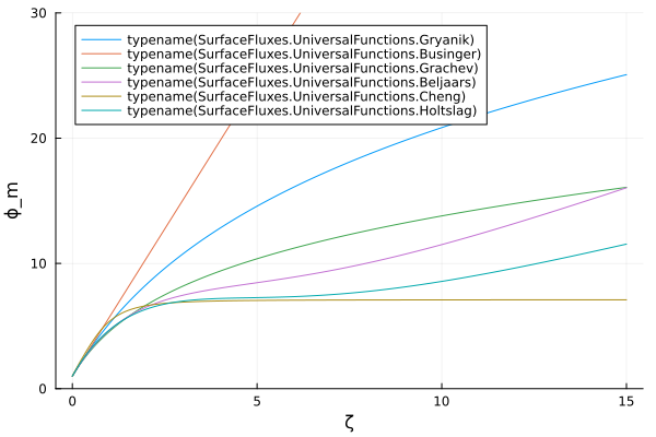
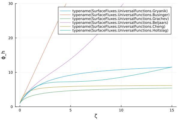
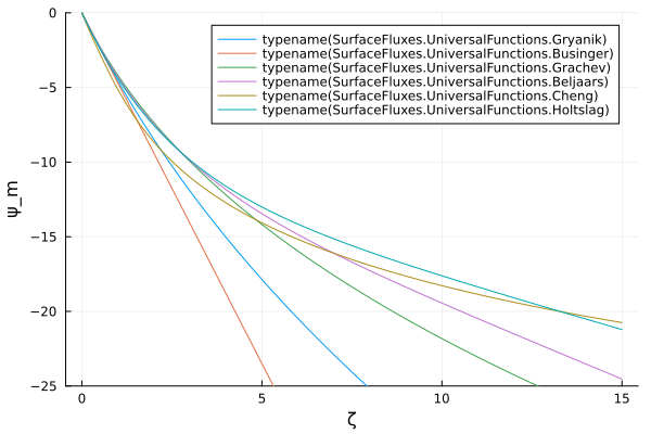
The following plots, in the style of Figures 1 and 2 of Gryanik et al. (2020), show the behavior of $\phi$ and $\psi$ in stable conditions with the default parameters of the package.

include("plot_universal_functions.jl")

Figures 1 & 2: Stable Conditions (Linear Scale)

Momentum stability function $\phi_m$ for stable conditions.

Heat stability function $\phi_h$ for stable conditions. Note that Gryanik has $\phi_h(0) = \text{Pr}_0 \approx 0.98$.

Momentum stability correction function $\psi_m$ for stable conditions.

Heat stability correction function $\psi_h$ for stable conditions.

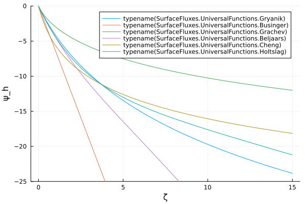
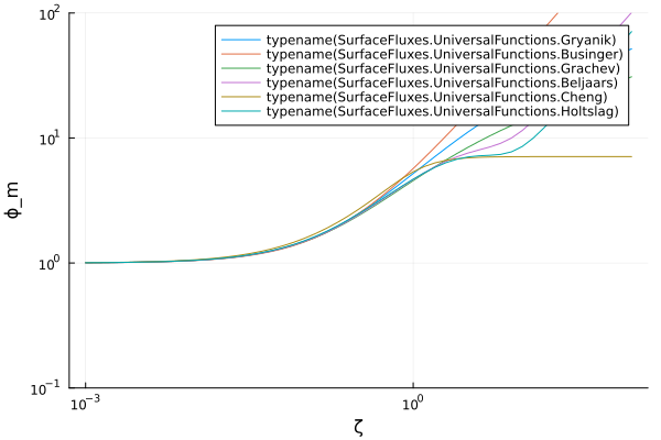
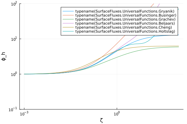
Figure 3: Extended Stability Range (Log-Log Scale)

Momentum stability function $\phi_m$ over extended stability range (log-log scale).

Heat stability function $\phi_h$ over extended stability range (log-log scale).

Comparison with Businger (1971)

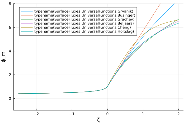
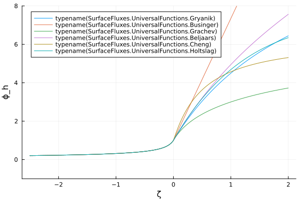
The classic Businger et al. (1971) curves for $\phi_m$ and $\phi_h$, along with the other parameterizations, across both stable and unstable conditions.

Momentum stability functions $\phi_m$ for stable and unstable conditions. For $\zeta < 0$, all parameterizations use the Businger-Dyer form.

Heat stability function $\phi_h$ for stable and unstable conditions. For $\zeta < 0$, all parameterizations use the Businger-Dyer shape $\text{Pr}_0 (1 - b_h \zeta)^{-1/2}$ with their own neutral Prandtl numbers (0.74 Businger, 0.98 Gryanik, 1 Grachev), so the curves differ by those factors.

References

• Businger, J. A., Wyngaard, J. C., Izumi, Y., & Bradley, E. F. (1971). Flux-profile relationships in the atmospheric surface layer. Journal of the Atmospheric Sciences, 28, 181-189. DOI: 10.1175/1520-0469(1971)028<0181:FPRITA>2.0.CO;2

• Högström, U. (1988). Non-dimensional wind and temperature profiles in the atmospheric surface layer: A re-evaluation. Boundary-Layer Meteorology, 42, 55–78. DOI: 10.1007/BF00119875

• Dyer, A. J. (1974). A review of flux-profile relationships. Boundary-Layer Meteorology, 7, 363-372. DOI: 10.1007/BF00240838

• Gryanik, V. M., Lüpkes, C., Grachev, A., and Sidorenko, D. (2020). New modified and extended stability functions for the stable boundary layer based on SHEBA and parametrizations of bulk transfer coefficients for climate models. Journal of the Atmospheric Sciences, 77, 2687–2716. DOI: 10.1175/JAS-D-19-0255.1

• Grachev, A. A., Andreas, E. L., Fairall, C. W., Guest, P. S., and Persson, P. O. G. (2007). SHEBA flux–profile relationships in the stable atmospheric boundary layer. Boundary-Layer Meteorology, 124, 315–333. DOI: 10.1007/s10546-007-9177-6

• Nishizawa, S., & Kitamura, Y. (2018). A surface flux scheme based on the Monin-Obukhov similarity for finite volume models. Journal of Advances in Modeling Earth Systems, 10, 3159–3175. DOI: 10.1029/2018MS001534