Atmospheric Temperature Profiles

Overview

The Thermodynamics.TemperatureProfiles module provides pre-defined atmospheric temperature profiles for testing and validation, and as reference states in atmosphere models. These profiles represent idealized atmospheric conditions used in climate modeling and testing.

Available Profiles

Three temperature profiles are currently available:

1. IsothermalProfile: Constant temperature with height
2. DecayingTemperatureProfile: Temperature decreases smoothly with height
3. DryAdiabaticProfile: Temperature follows dry adiabatic lapse rate

Usage

A profile is built once from a parameter set, then called at each altitude:

import Thermodynamics as TD
import Thermodynamics.Parameters as TP
import ClimaParams
FT = Float64
param_set = TP.ThermodynamicsParameters(FT)

profile = TD.TemperatureProfiles.DecayingTemperatureProfile{FT}(param_set) # construct
T, p = profile(param_set, FT(1000))    # evaluate at altitude z = 1000 m

(281.7873651934768, 89905.75006485406)

• The constructor takes param_set, a thermodynamic parameter set from ClimaParams.jl, plus optional profile parameters such as the surface temperature and scale heights.
• The resulting object is callable, taking param_set and the altitude z [m], and returning the temperature and pressure (T, p) there.

Isothermal Profile

A constant temperature profile, useful for testing thermodynamic calculations under uniform conditions.

import Thermodynamics as TD
import Plots
import ClimaParams as CP
import Thermodynamics.Parameters as TP
FT = Float64
param_set = TP.ThermodynamicsParameters(FT)
z = range(FT(0), stop = FT(2.5e4), length = 50);

isothermal = TD.TemperatureProfiles.IsothermalProfile(param_set, FT);
args = isothermal.(Ref(param_set), z);
T = first.(args);
p = last.(args);

p1 = Plots.plot(T, z./10^3, xlabel="Temperature [K]");
p2 = Plots.plot(p./10^3, z./10^3, xlabel="Pressure [kPa]");
Plots.plot(p1, p2, layout=(1,2), title="Isothermal", ylabel="z [km]");
Plots.savefig("isothermal.svg");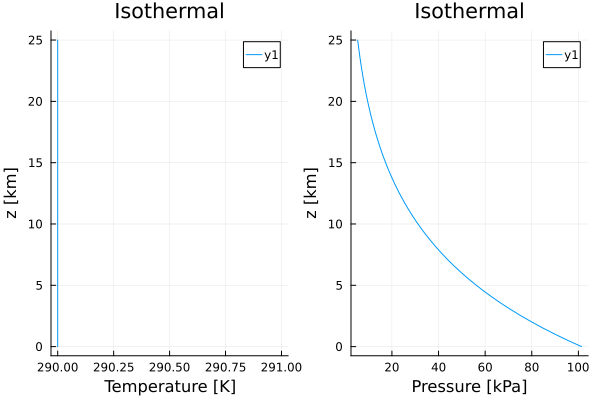

Decaying Temperature Profile

A profile where temperature decreases smoothly with height, representing typical atmospheric conditions.

import Thermodynamics as TD
import Plots
import ClimaParams as CP
import Thermodynamics.Parameters as TP
FT = Float64
param_set = TP.ThermodynamicsParameters(FT)
z = range(FT(0), stop = FT(2.5e4), length = 50);

decaying = TD.TemperatureProfiles.DecayingTemperatureProfile{FT}(param_set);
args = decaying.(Ref(param_set), z);
T = first.(args);
p = last.(args);

p1 = Plots.plot(T, z./10^3, xlabel="Temperature [K]");
p2 = Plots.plot(p./10^3, z./10^3, xlabel="Pressure [kPa]");
Plots.plot(p1, p2, layout=(1,2), ylabel="z [km]", title="Decaying");
Plots.savefig("decaying.svg");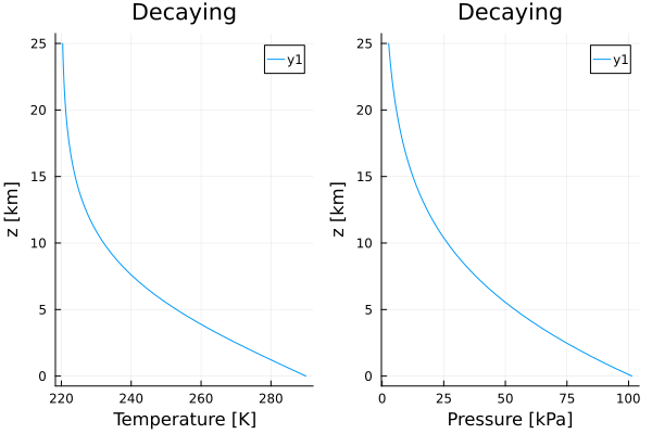

Dry Adiabatic Profile

A profile following the dry adiabatic lapse rate (potential temperature constant with height) down to some minimum temperature.

import Thermodynamics as TD
import Plots
import ClimaParams as CP
import Thermodynamics.Parameters as TP
FT = Float64
param_set = TP.ThermodynamicsParameters(FT)
z = range(FT(0), stop = FT(2.5e4), length = 50);

dry_adiabatic = TD.TemperatureProfiles.DryAdiabaticProfile{FT}(param_set);
args = dry_adiabatic.(Ref(param_set), z)
T = first.(args)
p = last.(args)
θ_dry = TD.potential_temperature_given_pressure.(Ref(param_set), T, p)

p1 = Plots.plot(T, z./10^3, xlabel="Temperature [K]");
p2 = Plots.plot(p./10^3, z./10^3, xlabel="Pressure [kPa]");
p3 = Plots.plot(θ_dry, z./10^3, xlabel="Potential temperature [K]");
Plots.plot(p1, p2, p3, layout=(1,3), ylabel="z [km]", title="Dry adiabatic");
Plots.savefig("dry_adiabatic.svg");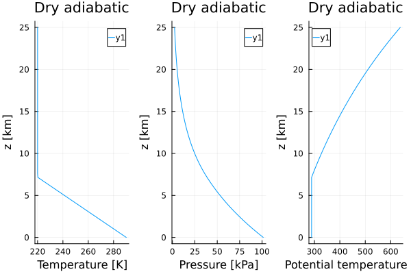

Applications

These temperature profiles are useful for:

• Testing thermodynamic calculations under controlled conditions
• Serving as reference states in atmosphere models
• Benchmarking performance across different atmospheric conditions
• Educational purposes to understand atmospheric thermodynamics

Extending the Module

Additional temperature profiles can be added by:

1. Creating a struct containing the parameters needed for the profile
2. Implementing a functor that takes (param_set, z) and returns (T, p)

Example structure:

# Skeleton: fill in the parameters and the (T, p) calculation
struct CustomProfile{FT} <: TD.TemperatureProfiles.TemperatureProfile{FT}
    # Profile parameters
end

function (profile::CustomProfile{FT})(param_set, z) where {FT}
    # Calculate T and p based on z
    return (T, p)
end