Performance and portability
ClimaCore runs on CPUs and on NVIDIA GPUs. This page describes how that portability is achieved, what the measured performance of the atmosphere built on it is, and where the costs are. The baseline numbers are those of [2], measured in September 2025 with the CliMA atmosphere (ClimaAtmos) in its moist baroclinic-wave configuration with 43 vertical levels. A more recent assessment on Derecho, after performance improvements, covers only a subset of those GPU measurements; no additional CPU scaling checks were run.
How portability is achieved
One kernel language. Model code is written as broadcast expressions over fields (Operators and broadcasting). On a CPU, a fused expression compiles to a loop; when the fields live on a ClimaComms.CUDADevice, the same expression compiles to a CUDA kernel through the ClimaCoreCUDAExt package extension, which loads when CUDA.jl is present. Every kernel assigns one thread per nodal point. Finite-difference kernels give a column to a group of threads along its levels; spectral-element kernels give each element slab a group of threads, one per node, pack several slabs into a thread block, and stage the slab in shared memory for the differentiation matrix. Kernels are specialized on the polynomial degree, so the loops over quadrature nodes unroll.
Device-agnostic data. A field's storage is an array whose type follows the device (Array or CuArray), and every grid, space, and operator is Adapt-able, so a model state moves between devices with ClimaCore.to_device. Halo exchanges for DSS and for DG face fluxes go through ClimaComms, which dispatches on the context type: a no-op on one process, MPI messages on many, GPU-aware where the MPI library supports it.
Memory layout. Field data is stored in one of the DataLayouts: VIJFH orders vertical level, the two horizontal node indices, the components of the value type, and the element index from fastest to slowest; VIJHF swaps the last two. The choice is a type parameter of the space (VIJH keyword), and the horizontal element index is the slowest so that one element is contiguous in memory. Elements are ordered along a space-filling curve (Topologies.spacefillingcurve) so that spatial neighbors are memory neighbors [39].
Precision. Every grid and field is parameterized on its float type; there are no separate Float32 and Float64 code paths. In the atmosphere's year-long conservation test, the relative drift of dry mass and total water is of order 10⁻¹³ in Float64 and 10⁻⁴ in Float32 [2].
Measured throughput and scaling
The table below mixes the published measurements of [2] (September 2025) with a September 2026 A100 re-check on Derecho. Hardware: NCAR's Derecho (four NVIDIA A100 GPUs per node), Google Cloud Platform NVIDIA H100 instances, and Caltech's Resnick cluster (two 32-core Intel Icelake CPUs per node, 16 MPI ranks per node).
The 2026 GPU figures overlay recent scaling measurements onto the published results. The 2026 runs cover only a subset of the published measurements: A100 strong scaling at 103 km and 51 km, and the two matching weak-scaling points (helem 30 on 1 GPU and helem 60 on 4 GPUs, about 5400 spectral elements per GPU). CPU scaling measurements remain the 2025 result.
| Quantity | Result |
|---|---|
| Weak scaling, 103 km → 6 km, 1 → 256 GPUs | Efficiency above 92% on GPUs; time per step stays near the 1-GPU value of 223 ms (Sep 2025) |
| Weak scaling on CPUs, 16 → 512 ranks | Efficiency above 98%, time per step near 2 s (Sep 2025; not re-run in 2026) |
| Strong scaling on GPUs | Efficiency above 95% while each GPU holds at least about 5400 spectral elements (Sep 2025); 2026 A100 re-check at 103 km and 51 km |
| Strong scaling on CPUs | About 80% at the highest resolution, up to 16 nodes (Sep 2025; not re-run in 2026) |
| Throughput at 25–50 km | More than 1 simulated year per day on a dozen to a few dozen GPUs |
| Throughput at 6 km, 256 H100 GPUs | 0.20 simulated years per day, with one-moment microphysics (Sep 2025) |
| Time per step at 51 km on 4 A100 GPUs | About 0.22 s (Sep 2025); 0.155 s (Sep 2026 A100 re-check) |
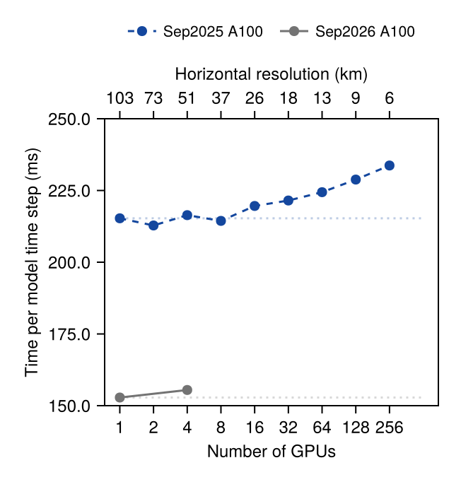
GPU weak scaling on Derecho A100s. Dashed navy: September 2025 published ladder (103 km to 6 km). Solid grey: September 2026 re-check at the two overlapping points (103 km on 1 GPU, 51 km on 4 GPUs). Dotted lines are the single-GPU time for each campaign.
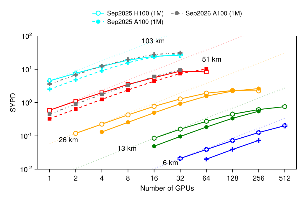
GPU strong scaling, simulated years per day. Hollow markers and solid lines: published results on H100 (GCP). Filled dashed lines: published results on A100 (Derecho). Grey solid lines: September 2026 A100 re-check at 103 km and 51 km. Dotted lines are ideal strong scaling from the 2025 H100 1-GPU (or few-GPU) points. The A100 curves at 26 km, 13 km, and 6 km — and all H100 curves — are 2025 published data. The GPU results use recent versions of ClimaCore and ClimaAtmos.
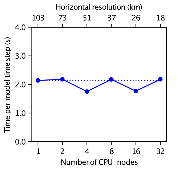
CPU weak scaling on Caltech's Resnick cluster (16 MPI ranks per node), published results from Yatunin et al. (2026). Time per model step stays near 2 s as the problem and rank count grow together from 1 to 32 nodes (103 km to 18 km), for efficiency above 98% from 16 to 512 ranks. The dotted line marks the single-node time. These CPU results use an earlier package version than the latest release.
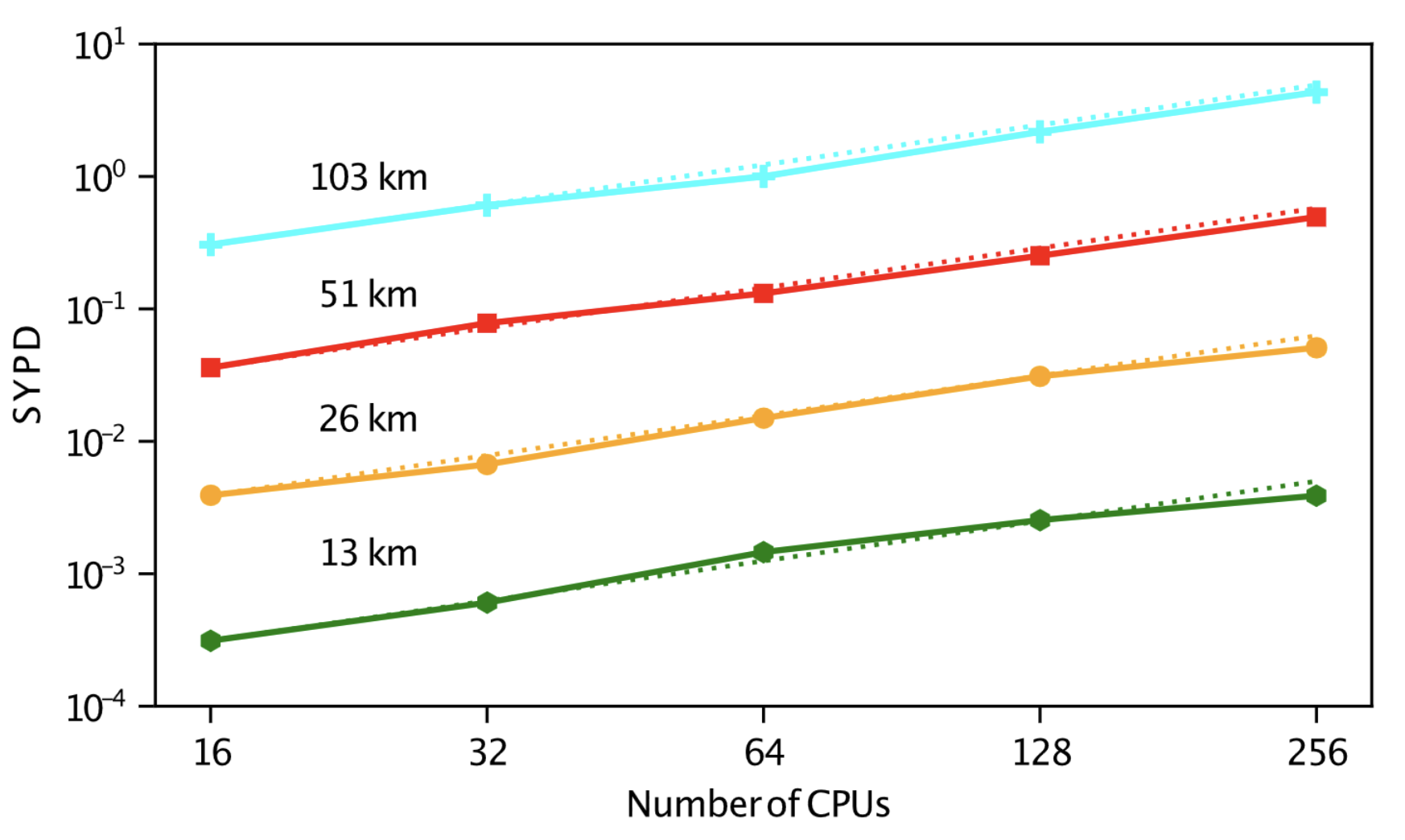
CPU strong scaling, simulated years per day against MPI rank count at fixed resolution, published results from Yatunin et al. (2026). Solid lines are measured throughput at 103 km, 51 km, 26 km, and 13 km; dotted lines are ideal strong scaling. Efficiency holds near 80% at the highest resolution up to 16 nodes (256 ranks). These CPU results use an earlier package version than the latest release.
The runs behind these figures are ClimaAtmos configurations. The GPU figures are drawn by plot_scaling_2026.jl in the ClimaAtmos repository. The 2025 published CPU plots were produced by miscellaneous/CPU_mbw_scaling_plots.jl. The moist baroclinic-wave benchmark itself is config/longrun_configs/longrun_moist_baroclinic_wave_he60.yml and its dry counterpart in the same directory. The earlier CI-oriented helpers remain at post_processing/plot_gpu_weak_scaling.jl, post_processing/plot_gpu_strong_scaling.jl, and post_processing/plot_gpu_scaling_utils.jl.
For context, the same paper compares against two other GPU dynamical cores: SCREAM (C++/Kokkos) reports 0.52 simulated years per day at 3.25 km on 1536 A100 GPUs [40], which after accounting for the roughly eightfold cost of halving the resolution is a comparable throughput per GPU, and Pace (Python) reports 3.98 s per step at about 50 km on 6 P100 GPUs [41]. H100 instances give the higher throughput at small GPU counts; Derecho's interconnect gives the better scaling efficiency, so several A100s match or exceed the H100 instances at high GPU counts. The point of the cloud measurements is access: a few dozen cloud GPUs run a global simulation at 25–50 km resolution faster than real time, without a supercomputer allocation.
Where the time goes
DSS is the only horizontal communication in a CG model and one of two exchanges (with the DG halo) in a DG model; everything else is element- or column-local. The vertical implicit solve is column-local and needs no communication. At fixed resolution, the per-step cost is dominated by kernel execution when each GPU holds thousands of elements and by launch and exchange latency when it holds few, which is the knee in the strong-scaling curves. Over-aggressive fusion of a long tendency into one kernel spills registers or exhausts shared memory and slows the kernel; the split points are chosen by measurement.
Four environment variables tune the GPU kernel launches; the Environment variables page lists them, and perf/sweep_kernel_configs.jl sweeps them. For writing new code that keeps these properties (no allocation in kernels, type stability, ifelse over branches), see the shared developer guides under docs/dev-guides/performance/.