Hydraulic functions

This tutorial shows how to specify the hydraulic functions used in Richard's equation. In particular, we show how to choose the formalism for matric potential and hydraulic conductivity, and how to make the hydraulic conductivity account for the presence of ice as well as the temperature dependence of the viscosity of liquid water.

ClimateMachine's Land model allows the user to pick between two hydraulics models, that of van Genuchten [1] or that of Brooks and Corey [2, 3]. The same model is consistently used for the matric potential and hydraulic conductivity.

Preliminary setup

External modules

using Plots

ClimateMachine modules

using ClimateMachine
using ClimateMachine.Land
using ClimateMachine.Land.SoilWaterParameterizations

FT = Float32;

Specifying a hydraulics model

The van Genuchten model requires two free parameters, α and n. A third parameter, m, is computed from n. Of these, only α carries units, of inverse meters. The Brooks and Corey model also uses two free parameters, ψ_b, the magnitude of the matric potential at saturation, and a constant M. ψ_b carries units of meters. The hydraulic conductivity requires an additional parameter, Ksat (m/s), which is the hydraulic conductivity in saturated soil. This parameter is the same between the two models for a given soil type, and is not stored in the hydraulics model, but rather as part of the SoilParamFunctions.

Below we show how to create two concrete examples of these hydraulics models, for sandy loam [1]. Note that the parameters chosen are a function of soil type.

vg_α = FT(7.5) # m^-1
vg_n = FT(1.89)
hydraulics = vanGenuchten{FT}(α = vg_α, n = vg_n)

ψ_sat = 0.09 # m
Mval = 0.228
hydraulics_bc = BrooksCorey{FT}(ψb = ψ_sat, m = Mval);

Matric Potential

The matric potential ψ represents how much water clings to soil. Drier soil holds onto water more tightly, making diffusion more difficult. As soil becomes wetter, the matric potential decreases in magnitude, making diffusion easier.

The van Genuchten expression for matric potential is $ψ = -\frac{1}{α} S_l^{-1/(nm)}\times (1-S_l^{1/m})^{1/n},$

and the Brooks and Corey expression is $ψ = -ψ_b S_l^{-M}.$

Here S_l is the effective saturation of liquid water, θ_l/ν, where ν is porosity of the soil. We neglect the residual pore space in the CliMA model.

In the CliMA code, we use multiple dispatch. With multiple dispatch, a function can have many ways of executing (called methods), depending on the type of the variables passed in. A simple example of multiple dispatch is the division operation. Integer division takes two numbers as input, and returns an integer - ignoring the decimal. Float division takes two numbers as input, and returns a floating point number, including the decimal. In Julia, we might write these as:

function division(a::Int, b::Int)
     return floor(Int, a/b)
end

function division(a::Float64, b::Float64)
     return a/b
end

We can see that division is now a function with two methods.

julia> division
division (generic function with 2 methods)

Now, using the same function signature, we can carry out integer division or floating point division, depending on the types of the arguments:

julia> division(1,2)
0

julia> division(1.0,2.0)
0.5

Here is a more pertinent example: hydraulics is of type vanGenuchten{Float32} based on our choice of FT:

julia> typeof(hydraulics)
vanGenuchten{Float32}

but meanwhile,

julia> typeof(hydraulics_bc)
BrooksCorey{Float32}

The function matric_potential will execute different methods depending on if we pass a hydraulics model of type vanGenuchten or BrooksCorey. In both cases, it will return the correct value for ψ.

Let's plot the matric potential as a function of the effective saturation S_l = θ_l/ν, which can range from zero to one.

S_l = FT.(0.01:0.01:0.99)
ψ = matric_potential.(Ref(hydraulics), S_l)
ψ_bc = matric_potential.(Ref(hydraulics_bc), S_l)
plot(
    S_l,
    log10.(-ψ),
    xlabel = "effective saturation",
    ylabel = "Log10(|ψ|)",
    label = "van Genuchten",
)
plot!(S_l, log10.(-ψ_bc), label = "Brooks and Corey")
savefig("bc_vg_matric_potential.png")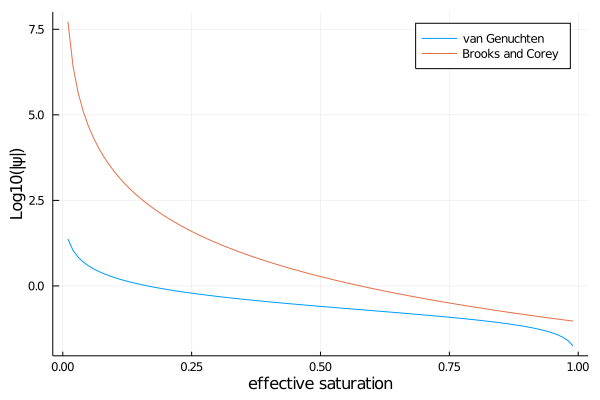

The steep slope in ψ near saturated and completely dry soil are part of the reason why Richard's equation is such a challenging numerical problem.

Hydraulic conductivity

The hydraulic conductivity is a more complex function than the matric potential, as it depends on the temperature of the water, the volumetric ice fraction, and the volumetric liquid water fraction. It also depends on the hydraulics model chosen.

We represent the hydraulic conductivity K as the product of four factors: Ksat, an impedance_factor (which accounts for the effect of ice on conductivity) a viscosity_factor (which accounts for the effect of temperature on the viscosity of liquid water, and how that in turn affects conductivity) and a moisture_factor (which accounts for the effect of liquid water, and is determined by the hydraulics model).

Let's start with ice and temperature independence, but moisture dependence. Below we choose additional parameters, consistent with the hydraulics parameters for sandy loam [1].

ν = FT(0.41)
Ksat = FT(4.42 / (3600 * 100))
moisture_choice = MoistureDependent{FT}()
viscosity_choice = ConstantViscosity{FT}()
impedance_choice = NoImpedance{FT}();

We are going to calculate K = Ksat × viscosity_factor × impedance_factor × moisture_factor. In the code, each of these factors is a function with multiple methods, except for Ksat. Our function hydraulic_conductivity calls each of these functions in turn, and these functions use multiple dispatch to provide the correct value for K.

Like we defined new type classes for vanGenuchten{FT} and BrooksCorey{FT}, we also created new type classes for the impedance choice, the viscosity choice, and the moisture choice. For example, the function called viscosity_factor, when passed an object of type ConstantViscosity{FT}, executes a method that always returns 1. The same is true for the function impedance_factor, using the type NoImpedance{FT}, and for moisture_factor, using the type MoistureIndependent{FT}.

In the case where the moisture_factor = MoistureDependent{FT}(), either the van Genuchten or Brooks and Corey expression is used based on the type of hydraulics model passed.

The moisture_factor for the van Genuchten model is (denoting it as $K_m$)

$K_m = \sqrt{S_l}[1-(1-S_l^{1/m})^m]^2,$

for $S_l < 1$,

and for the Brooks and Corey model it is

$K_m = S_l^{2M+3},$

also for $S_l<1$. When $S_l\geq 1$, $K_m = 1$ for each model.

One side effect of this flexibility is that hydraulic_conductivity requires all the arguments it could possibly need passed to it, which is why here we must supply a value T and θ_i, even though they are not used in this particular example.

T = FT(0.0)
θ_i = FT(0.0)

K =
    Ksat .*
    hydraulic_conductivity.(
        Ref(impedance_choice),
        Ref(viscosity_choice),
        Ref(moisture_choice),
        Ref(hydraulics),
        Ref(θ_i),
        Ref(ν),
        Ref(T),
        S_l,
    );

Let's also compute K when we include the effects of temperature and ice on the hydraulic conductivity. In the cases where a TemperatureDependentViscosity{FT} or IceImpedance{FT} type is passed, the correct factors are calculated, based on the temperature T and volumetric ice fraction θ_i. In these cases, the viscosity_factor, denoted here as $K_v$, evaluates as:

$K_v = e^{\gamma(T-T_{ref})},$

where $\gamma = 0.0264 \mbox{K}^{-1}$ is an empirical factor, and $T_{ref} = 288$ K, and the impedance_factor, denoted $K_i$, evaluates as:

$K_i = 10^{-\Omega f_i}$

where $\Omega = 7$ is an empirical factor and $f_i$ is the ratio of the volumetric ice fraction to total volumetric water fraction [5].

viscosity_choice_T = TemperatureDependentViscosity{FT}()
T = FT(300.0)
K_T =
    Ksat .*
    hydraulic_conductivity.(
        Ref(impedance_choice),
        Ref(viscosity_choice_T),
        Ref(moisture_choice),
        Ref(hydraulics),
        Ref(θ_i),
        Ref(ν),
        Ref(T),
        S_l,
    )
ice_impedance_I = IceImpedance{FT}()
θ_i = FT(0.1)
S_i = θ_i / ν;

The total volumetric water fraction cannot exceed unity, so the effective liquid water saturation should have a max of 1-S_i.

S_l_accounting_for_ice = FT.(0.01:0.01:(0.99 - S_i))
K_i =
    Ksat .*
    hydraulic_conductivity.(
        Ref(ice_impedance_I),
        Ref(viscosity_choice),
        Ref(moisture_choice),
        Ref(hydraulics),
        Ref(θ_i),
        Ref(ν),
        Ref(T),
        S_l_accounting_for_ice,
    )
plot(
    S_l,
    log10.(K),
    xlabel = "total effective saturation, (θ_i+θ_l)/ν",
    ylabel = "Log10(K)",
    label = "Base case",
    legend = :bottomright,
)
plot!(S_l, log10.(K_T), label = "Temperature Dependent Viscosity; no ice")
plot!(
    S_l_accounting_for_ice .+ S_i,
    log10.(K_i),
    label = "Ice Impedance; S_i=0.24",
)
savefig("T_ice_K.png")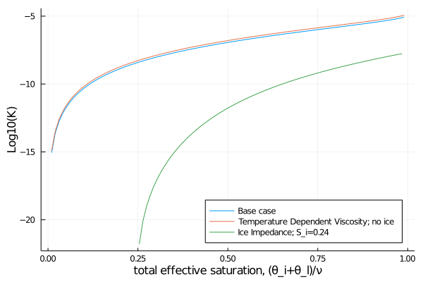

If the user is not considering phase transitions and does not add in Freeze/Thaw source terms, the default is for zero ice in the model, for all time and space. In this case the ice impedance factor evaluates to 1 regardless of which type is passed.

We can also look and see how the Brooks and Corey moisture factor differs from the van Genuchten moisture factor by changing the hydraulics model passed:

T = FT(0.0)
θ_i = FT(0.0)

K_bc =
    Ksat .*
    hydraulic_conductivity.(
        Ref(impedance_choice),
        Ref(viscosity_choice),
        Ref(moisture_choice),
        Ref(hydraulics_bc),
        Ref(θ_i),
        Ref(ν),
        Ref(T),
        S_l,
    )
plot(
    S_l,
    log10.(K),
    xlabel = "effective saturation",
    ylabel = "Log10(K)",
    label = "van Genuchten",
)
plot!(
    S_l,
    log10.(K_bc),
    xlabel = "effective saturation",
    ylabel = "Log10(K)",
    label = "Brooks and Corey",
)
savefig("bc_vg_k.png")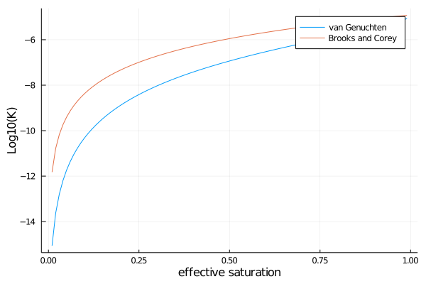

Other features

The user also has the choice of making the conductivity constant by choosing MoistureIndependent{FT}() along with ConstantViscosity{FT}() and NoImpedance{FT}() . This is useful for debugging!

no_moisture_dependence = MoistureIndependent{FT}()
K_constant =
    Ksat .*
    hydraulic_conductivity.(
        Ref(impedance_choice),
        Ref(viscosity_choice),
        Ref(no_moisture_dependence),
        Ref(hydraulics),
        Ref(θ_i),
        Ref(ν),
        Ref(T),
        S_l,
    );

julia> unique(K_constant)
1-element Array{Float32,1}:
 1.2277777f-5

Note that choosing this option does not mean the matric potential is constant, as a hydraulics model is still required and employed.

And, lastly, you might be wondering why we left Ksat out of the function for hydraulic_conductivity. It turns out it is also useful for debugging to be able to turn off the diffusion of water, by setting Ksat = 0.

References

[1] van Genuchten, M. T. (1980), A closed-form equation for predicting the hydraulic conductivity of unsaturated soils, Soil Sci. Soc. Amer. J., pp. 892–898.

[2] Brooks, R. J., and A. T. Corey (1964), Hydraulic properties of porous media.

[3] Corey, A. T. (1977), Mechanics of Heterogeneous Fluids in Porous Media, Water Resources Publication, Fort Collins, CO.

[4] Bonan, G. (2019), Climate Change and Terrestrial Ecoystem Modeling, Cambridge Univ. Press, Cambridge, UK, and New York, NY, USA. Chapter 8, Page 120

[5] Lundin, L.-C. (1990), Hydraulic properties in an operational model of frozen soil, J. Hydrol., 118, 289–310.

This page was generated using Literate.jl.