Baroclinic adjustment

In this example, we simulate the evolution and equilibration of a baroclinically unstable front.

Install dependencies

First let's make sure we have all required packages installed.

using Pkg
pkg"add Oceananigans, CairoMakie"

using Oceananigans
using Oceananigans.Units

Grid

We use a three-dimensional channel that is periodic in the x direction:

Lx = 1000kilometers # east-west extent [m]
Ly = 1000kilometers # north-south extent [m]
Lz = 1kilometers    # depth [m]

grid = RectilinearGrid(size = (48, 48, 8),
                       x = (0, Lx),
                       y = (-Ly/2, Ly/2),
                       z = (-Lz, 0),
                       topology = (Periodic, Bounded, Bounded))

48×48×8 RectilinearGrid{Float64, Periodic, Bounded, Bounded} on CPU with 3×3×3 halo
├── Periodic x ∈ [0.0, 1.0e6)          regularly spaced with Δx=20833.3
├── Bounded  y ∈ [-500000.0, 500000.0] regularly spaced with Δy=20833.3
└── Bounded  z ∈ [-1000.0, 0.0]        regularly spaced with Δz=125.0

Model

We built a HydrostaticFreeSurfaceModel with an ImplicitFreeSurface solver. Regarding Coriolis, we use a beta-plane centered at 45° South.

model = HydrostaticFreeSurfaceModel(; grid,
                                    coriolis = BetaPlane(latitude = -45),
                                    buoyancy = BuoyancyTracer(),
                                    tracers = :b,
                                    momentum_advection = WENO(),
                                    tracer_advection = WENO())

HydrostaticFreeSurfaceModel{CPU, RectilinearGrid}(time = 0 seconds, iteration = 0)
├── grid: 48×48×8 RectilinearGrid{Float64, Periodic, Bounded, Bounded} on CPU with 3×3×3 halo
├── timestepper: QuasiAdamsBashforth2TimeStepper
├── tracers: b
├── closure: Nothing
├── buoyancy: BuoyancyTracer with ĝ = NegativeZDirection()
├── free surface: ImplicitFreeSurface with gravitational acceleration 9.80665 m s⁻²
│   └── solver: FFTImplicitFreeSurfaceSolver
├── advection scheme: 
│   ├── momentum: WENO reconstruction order 5
│   └── b: WENO reconstruction order 5
└── coriolis: BetaPlane{Float64}

We start our simulation from rest with a baroclinically unstable buoyancy distribution. We use ramp(y, Δy), defined below, to specify a front with width Δy and horizontal buoyancy gradient M². We impose the front on top of a vertical buoyancy gradient N² and a bit of noise.

"""
    ramp(y, Δy)

Linear ramp from 0 to 1 between -Δy/2 and +Δy/2.

For example:
```
            y < -Δy/2 => ramp = 0
    -Δy/2 < y < -Δy/2 => ramp = y / Δy
            y >  Δy/2 => ramp = 1
```
"""
ramp(y, Δy) = min(max(0, y/Δy + 1/2), 1)

N² = 1e-5 # [s⁻²] buoyancy frequency / stratification
M² = 1e-7 # [s⁻²] horizontal buoyancy gradient

Δy = 100kilometers # width of the region of the front
Δb = Δy * M²       # buoyancy jump associated with the front
ϵb = 1e-2 * Δb     # noise amplitude

bᵢ(x, y, z) = N² * z + Δb * ramp(y, Δy) + ϵb * randn()

set!(model, b=bᵢ)

Let's visualize the initial buoyancy distribution.

using CairoMakie

# Build coordinates with units of kilometers
x, y, z = 1e-3 .* nodes(grid, (Center(), Center(), Center()))

b = model.tracers.b

fig, ax, hm = heatmap(y, z, interior(b)[1, :, :],
                      colormap=:deep,
                      axis = (xlabel = "y [km]",
                              ylabel = "z [km]",
                              title = "b(x=0, y, z, t=0)",
                              titlesize = 24))

Colorbar(fig[1, 2], hm, label = "[m s⁻²]")

fig

Simulation

Now let's build a Simulation.

simulation = Simulation(model, Δt=20minutes, stop_time=20days)

Simulation of HydrostaticFreeSurfaceModel{CPU, RectilinearGrid}(time = 0 seconds, iteration = 0)
├── Next time step: 20 minutes
├── Elapsed wall time: 0 seconds
├── Wall time per iteration: NaN days
├── Stop time: 20 days
├── Stop iteration : Inf
├── Wall time limit: Inf
├── Callbacks: OrderedDict with 4 entries:
│   ├── stop_time_exceeded => Callback of stop_time_exceeded on IterationInterval(1)
│   ├── stop_iteration_exceeded => Callback of stop_iteration_exceeded on IterationInterval(1)
│   ├── wall_time_limit_exceeded => Callback of wall_time_limit_exceeded on IterationInterval(1)
│   └── nan_checker => Callback of NaNChecker for u on IterationInterval(100)
├── Output writers: OrderedDict with no entries
└── Diagnostics: OrderedDict with no entries

We add a TimeStepWizard callback to adapt the simulation's time-step,

conjure_time_step_wizard!(simulation, IterationInterval(20), cfl=0.2, max_Δt=20minutes)

Also, we add a callback to print a message about how the simulation is going,

using Printf

wall_clock = Ref(time_ns())

function print_progress(sim)
    u, v, w = model.velocities
    progress = 100 * (time(sim) / sim.stop_time)
    elapsed = (time_ns() - wall_clock[]) / 1e9

    @printf("[%05.2f%%] i: %d, t: %s, wall time: %s, max(u): (%6.3e, %6.3e, %6.3e) m/s, next Δt: %s\n",
            progress, iteration(sim), prettytime(sim), prettytime(elapsed),
            maximum(abs, u), maximum(abs, v), maximum(abs, w), prettytime(sim.Δt))

    wall_clock[] = time_ns()

    return nothing
end

add_callback!(simulation, print_progress, IterationInterval(100))

Diagnostics/Output

Here, we save the buoyancy, $b$, at the edges of our domain as well as the zonal ($x$) average of buoyancy.

u, v, w = model.velocities
ζ = ∂x(v) - ∂y(u)
B = Average(b, dims=1)
U = Average(u, dims=1)
V = Average(v, dims=1)

filename = "baroclinic_adjustment"
save_fields_interval = 0.5day

slicers = (east = (grid.Nx, :, :),
           north = (:, grid.Ny, :),
           bottom = (:, :, 1),
           top = (:, :, grid.Nz))

for side in keys(slicers)
    indices = slicers[side]

    simulation.output_writers[side] = JLD2OutputWriter(model, (; b, ζ);
                                                       filename = filename * "_$(side)_slice",
                                                       schedule = TimeInterval(save_fields_interval),
                                                       overwrite_existing = true,
                                                       indices)
end

simulation.output_writers[:zonal] = JLD2OutputWriter(model, (; b=B, u=U, v=V);
                                                     filename = filename * "_zonal_average",
                                                     schedule = TimeInterval(save_fields_interval),
                                                     overwrite_existing = true)

JLD2OutputWriter scheduled on TimeInterval(12 hours):
├── filepath: ./baroclinic_adjustment_zonal_average.jld2
├── 3 outputs: (b, u, v)
├── array type: Array{Float64}
├── including: [:grid, :coriolis, :buoyancy, :closure]
├── file_splitting: NoFileSplitting
└── file size: 29.3 KiB

Now we're ready to run.

@info "Running the simulation..."

run!(simulation)

@info "Simulation completed in " * prettytime(simulation.run_wall_time)

[ Info: Running the simulation...
[ Info: Initializing simulation...
[00.00%] i: 0, t: 0 seconds, wall time: 27.937 seconds, max(u): (0.000e+00, 0.000e+00, 0.000e+00) m/s, next Δt: 20 minutes
[ Info:     ... simulation initialization complete (35.498 seconds)
[ Info: Executing initial time step...
[ Info:     ... initial time step complete (28.818 seconds).
[06.94%] i: 100, t: 1.389 days, wall time: 1.021 minutes, max(u): (1.254e-01, 1.238e-01, 1.487e-03) m/s, next Δt: 20 minutes
[13.89%] i: 200, t: 2.778 days, wall time: 4.867 seconds, max(u): (2.141e-01, 1.792e-01, 1.755e-03) m/s, next Δt: 20 minutes
[20.83%] i: 300, t: 4.167 days, wall time: 4.850 seconds, max(u): (2.825e-01, 2.414e-01, 1.742e-03) m/s, next Δt: 20 minutes
[27.78%] i: 400, t: 5.556 days, wall time: 4.799 seconds, max(u): (3.664e-01, 3.336e-01, 1.934e-03) m/s, next Δt: 20 minutes
[34.72%] i: 500, t: 6.944 days, wall time: 5.210 seconds, max(u): (4.622e-01, 5.312e-01, 2.126e-03) m/s, next Δt: 20 minutes
[41.67%] i: 600, t: 8.333 days, wall time: 4.847 seconds, max(u): (6.447e-01, 7.784e-01, 3.024e-03) m/s, next Δt: 20 minutes
[48.61%] i: 700, t: 9.722 days, wall time: 4.787 seconds, max(u): (8.423e-01, 1.169e+00, 3.334e-03) m/s, next Δt: 20 minutes
[55.56%] i: 800, t: 11.111 days, wall time: 4.880 seconds, max(u): (1.101e+00, 1.290e+00, 4.001e-03) m/s, next Δt: 20 minutes
[62.50%] i: 900, t: 12.500 days, wall time: 4.798 seconds, max(u): (1.451e+00, 1.297e+00, 4.936e-03) m/s, next Δt: 20 minutes
[69.44%] i: 1000, t: 13.889 days, wall time: 5.099 seconds, max(u): (1.547e+00, 1.271e+00, 3.891e-03) m/s, next Δt: 20 minutes
[76.39%] i: 1100, t: 15.278 days, wall time: 4.843 seconds, max(u): (1.415e+00, 1.157e+00, 3.574e-03) m/s, next Δt: 20 minutes
[83.33%] i: 1200, t: 16.667 days, wall time: 7.710 seconds, max(u): (1.486e+00, 1.024e+00, 2.779e-03) m/s, next Δt: 20 minutes
[90.28%] i: 1300, t: 18.056 days, wall time: 6.246 seconds, max(u): (1.346e+00, 9.755e-01, 2.176e-03) m/s, next Δt: 20 minutes
[97.22%] i: 1400, t: 19.444 days, wall time: 9.954 seconds, max(u): (1.355e+00, 9.891e-01, 4.397e-03) m/s, next Δt: 20 minutes
[ Info: Simulation is stopping after running for 2.469 minutes.
[ Info: Simulation time 20 days equals or exceeds stop time 20 days.
[ Info: Simulation completed in 2.472 minutes

Visualization

All that's left is to make a pretty movie. Actually, we make two visualizations here. First, we illustrate how to make a 3D visualization with Makie's Axis3 and Makie.surface. Then we make a movie in 2D. We use CairoMakie in this example, but note that using GLMakie is more convenient on a system with OpenGL, as figures will be displayed on the screen.

using CairoMakie

Three-dimensional visualization

We load the saved buoyancy output on the top, bottom, north, and east surface as FieldTimeSerieses.

filename = "baroclinic_adjustment"

sides = keys(slicers)

slice_filenames = NamedTuple(side => filename * "_$(side)_slice.jld2" for side in sides)

b_timeserieses = (east   = FieldTimeSeries(slice_filenames.east, "b"),
                  north  = FieldTimeSeries(slice_filenames.north, "b"),
                  bottom = FieldTimeSeries(slice_filenames.bottom, "b"),
                  top    = FieldTimeSeries(slice_filenames.top, "b"))

B_timeseries = FieldTimeSeries(filename * "_zonal_average.jld2", "b")

times = B_timeseries.times
grid = B_timeseries.grid

48×48×8 RectilinearGrid{Float64, Periodic, Bounded, Bounded} on CPU with 3×3×3 halo
├── Periodic x ∈ [0.0, 1.0e6)          regularly spaced with Δx=20833.3
├── Bounded  y ∈ [-500000.0, 500000.0] regularly spaced with Δy=20833.3
└── Bounded  z ∈ [-1000.0, 0.0]        regularly spaced with Δz=125.0

We build the coordinates. We rescale horizontal coordinates to kilometers.

xb, yb, zb = nodes(b_timeserieses.east)

xb = xb ./ 1e3 # convert m -> km
yb = yb ./ 1e3 # convert m -> km

Nx, Ny, Nz = size(grid)
x_xz = repeat(x, 1, Nz)
y_xz_north = y[end] * ones(Nx, Nz)
z_xz = repeat(reshape(z, 1, Nz), Nx, 1)

x_yz_east = x[end] * ones(Ny, Nz)
y_yz = repeat(y, 1, Nz)
z_yz = repeat(reshape(z, 1, Nz), grid.Ny, 1)

x_xy = x
y_xy = y
z_xy_top = z[end] * ones(grid.Nx, grid.Ny)
z_xy_bottom = z[1] * ones(grid.Nx, grid.Ny)

Then we create a 3D axis. We use zonal_slice_displacement to control where the plot of the instantaneous zonal average flow is located.

fig = Figure(size = (1600, 800))

zonal_slice_displacement = 1.2

ax = Axis3(fig[2, 1],
           aspect=(1, 1, 1/5),
           xlabel = "x (km)",
           ylabel = "y (km)",
           zlabel = "z (m)",
           xlabeloffset = 100,
           ylabeloffset = 100,
           zlabeloffset = 100,
           limits = ((x[1], zonal_slice_displacement * x[end]), (y[1], y[end]), (z[1], z[end])),
           elevation = 0.45,
           azimuth = 6.8,
           xspinesvisible = false,
           zgridvisible = false,
           protrusions = 40,
           perspectiveness = 0.7)

Axis3()

We use data from the final savepoint for the 3D plot. Note that this plot can easily be animated by using Makie's Observable. To dive into Observables, check out Makie.jl's Documentation.

n = length(times)

41

Now let's make a 3D plot of the buoyancy and in front of it we'll use the zonally-averaged output to plot the instantaneous zonal-average of the buoyancy.

b_slices = (east   = interior(b_timeserieses.east[n], 1, :, :),
            north  = interior(b_timeserieses.north[n], :, 1, :),
            bottom = interior(b_timeserieses.bottom[n], :, :, 1),
            top    = interior(b_timeserieses.top[n], :, :, 1))

# Zonally-averaged buoyancy
B = interior(B_timeseries[n], 1, :, :)

clims = 1.1 .* extrema(b_timeserieses.top[n][:])

kwargs = (colorrange=clims, colormap=:deep)
surface!(ax, x_yz_east, y_yz, z_yz;    color = b_slices.east, kwargs...)
surface!(ax, x_xz, y_xz_north, z_xz;   color = b_slices.north, kwargs...)
surface!(ax, x_xy, y_xy, z_xy_bottom ; color = b_slices.bottom, kwargs...)
surface!(ax, x_xy, y_xy, z_xy_top;     color = b_slices.top, kwargs...)

sf = surface!(ax, zonal_slice_displacement .* x_yz_east, y_yz, z_yz; color = B, kwargs...)

contour!(ax, y, z, B; transformation = (:yz, zonal_slice_displacement * x[end]),
         levels = 15, linewidth = 2, color = :black)

Colorbar(fig[2, 2], sf, label = "m s⁻²", height = Relative(0.4), tellheight=false)

title = "Buoyancy at t = " * string(round(times[n] / day, digits=1)) * " days"
fig[1, 1:2] = Label(fig, title; fontsize = 24, tellwidth = false, padding = (0, 0, -120, 0))

rowgap!(fig.layout, 1, Relative(-0.2))
colgap!(fig.layout, 1, Relative(-0.1))

save("baroclinic_adjustment_3d.png", fig)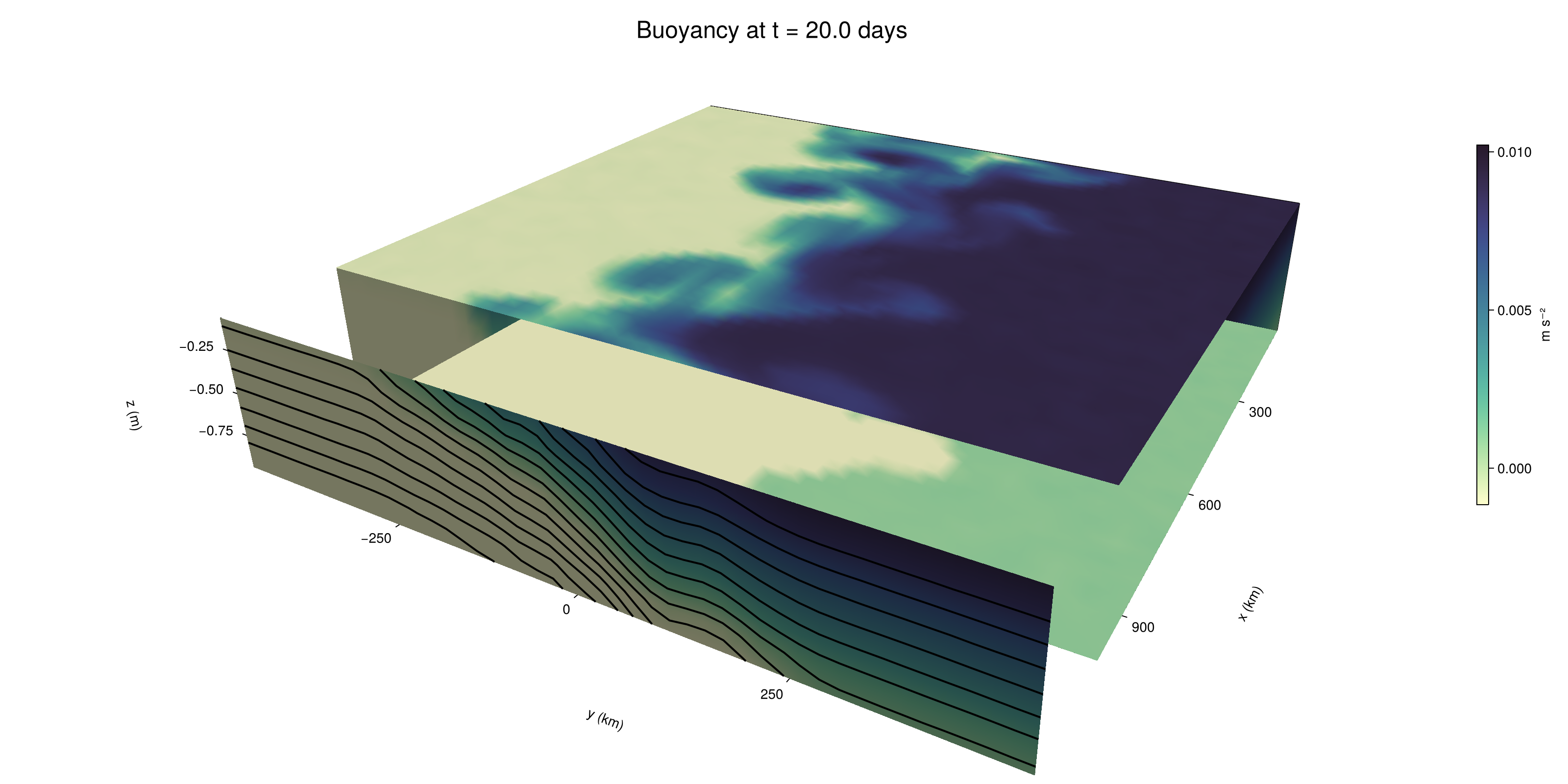

Two-dimensional movie

We make a 2D movie that shows buoyancy $b$ and vertical vorticity $ζ$ at the surface, as well as the zonally-averaged zonal and meridional velocities $U$ and $V$ in the $(y, z)$ plane. First we load the FieldTimeSeries and extract the additional coordinates we'll need for plotting

ζ_timeseries = FieldTimeSeries(slice_filenames.top, "ζ")
U_timeseries = FieldTimeSeries(filename * "_zonal_average.jld2", "u")
B_timeseries = FieldTimeSeries(filename * "_zonal_average.jld2", "b")
V_timeseries = FieldTimeSeries(filename * "_zonal_average.jld2", "v")

xζ, yζ, zζ = nodes(ζ_timeseries)
yv = ynodes(V_timeseries)

xζ = xζ ./ 1e3 # convert m -> km
yζ = yζ ./ 1e3 # convert m -> km
yv = yv ./ 1e3 # convert m -> km

49-element Vector{Float64}:
 -500.0
 -479.1666666666667
 -458.3333333333333
 -437.5
 -416.6666666666667
 -395.8333333333333
 -375.0
 -354.1666666666667
 -333.3333333333333
 -312.5
 -291.6666666666667
 -270.8333333333333
 -250.0
 -229.16666666666666
 -208.33333333333334
 -187.5
 -166.66666666666666
 -145.83333333333334
 -125.0
 -104.16666666666667
  -83.33333333333333
  -62.5
  -41.666666666666664
  -20.833333333333332
    0.0
   20.833333333333332
   41.666666666666664
   62.5
   83.33333333333333
  104.16666666666667
  125.0
  145.83333333333334
  166.66666666666666
  187.5
  208.33333333333334
  229.16666666666666
  250.0
  270.8333333333333
  291.6666666666667
  312.5
  333.3333333333333
  354.1666666666667
  375.0
  395.8333333333333
  416.6666666666667
  437.5
  458.3333333333333
  479.1666666666667
  500.0

Next, we set up a plot with 4 panels. The top panels are large and square, while the bottom panels get a reduced aspect ratio through rowsize!.

set_theme!(Theme(fontsize=24))

fig = Figure(size=(1800, 1000))

axb = Axis(fig[1, 2], xlabel="x (km)", ylabel="y (km)", aspect=1)
axζ = Axis(fig[1, 3], xlabel="x (km)", ylabel="y (km)", aspect=1, yaxisposition=:right)

axu = Axis(fig[2, 2], xlabel="y (km)", ylabel="z (m)")
axv = Axis(fig[2, 3], xlabel="y (km)", ylabel="z (m)", yaxisposition=:right)

rowsize!(fig.layout, 2, Relative(0.3))

To prepare a plot for animation, we index the timeseries with an Observable,

n = Observable(1)

b_top = @lift interior(b_timeserieses.top[$n], :, :, 1)
ζ_top = @lift interior(ζ_timeseries[$n], :, :, 1)
U = @lift interior(U_timeseries[$n], 1, :, :)
V = @lift interior(V_timeseries[$n], 1, :, :)
B = @lift interior(B_timeseries[$n], 1, :, :)

Observable([-0.009385317690602192 -0.008129038871684896 -0.006899638231146904 -0.005644616981664979 -0.004358790303257574 -0.003146977158134725 -0.0018740536913947293 -0.0006532429559926812; -0.009367595230292862 -0.008121849089508764 -0.006897297027347112 -0.00564807231947101 -0.004389002601211449 -0.003127880707542763 -0.0018894505128395158 -0.0006124143863898155; -0.009382341670424078 -0.008135326218309969 -0.006888909280069498 -0.005626875368164919 -0.004382915800081711 -0.0031217649326118224 -0.0018881536997935114 -0.000613032849379354; -0.009390496671510623 -0.008115664703983566 -0.006876746291688732 -0.0056048387128211155 -0.00434071894973458 -0.003107486719608579 -0.001882208951160394 -0.0006470504111457308; -0.009386853769577297 -0.008128718116264077 -0.006854573428535338 -0.005627305026689139 -0.004375390169847938 -0.0031441034195098215 -0.0018899854309792354 -0.0006165820193308865; -0.0093771421913736 -0.008102119759587413 -0.006868489396212649 -0.005625021196004315 -0.004366337628640339 -0.003146074933690779 -0.0018634744786260836 -0.0006296831118784811; -0.009378341603340092 -0.008135587704644618 -0.006895008175021621 -0.005635109341146125 -0.004392833046452854 -0.0031235614886128086 -0.0018988391666413835 -0.0006204676028629434; -0.009352212164292875 -0.008119804601933697 -0.0068651142336132705 -0.005598377275865328 -0.004400589932383253 -0.003115153268386395 -0.0018805605300711728 -0.0006517860669866454; -0.009406453408772523 -0.008133641848544001 -0.00686471365390605 -0.005634798181533449 -0.004350222234553903 -0.0031296396855265683 -0.0018736333109621755 -0.0006185209539741589; -0.009391140303066167 -0.008119154610382439 -0.0068842778970142 -0.005616905750280184 -0.00439375220265667 -0.0031313310718323636 -0.001872440792455207 -0.0006352831796260732; -0.009383390952005041 -0.00812922539201676 -0.00689909755167314 -0.0056397731945076685 -0.004394708145123651 -0.0031127302676311423 -0.0018624660012144208 -0.0006106994493673995; -0.009383626459695683 -0.008143011069522555 -0.006850772033181518 -0.0056336728347003455 -0.004365751778694134 -0.0031373140453857078 -0.0018852022021434635 -0.0006607195719167749; -0.009400699543216966 -0.008147113027539019 -0.0068787413262588705 -0.005608771685060067 -0.004374494164084744 -0.00311317654086056 -0.0018724740334390571 -0.000647964240692181; -0.009381292622452582 -0.008136263899327806 -0.006864932479437491 -0.005622888801540577 -0.004375440768716411 -0.003128647112241092 -0.0018695431214960222 -0.0006268220346660423; -0.009386859985351497 -0.008131996076485777 -0.006858898858462886 -0.005632468323140495 -0.0043747531771868384 -0.0031520872973105664 -0.0018631193856228987 -0.0006428215356176725; -0.009377634130161393 -0.008133922218547947 -0.006891662299381142 -0.0056299012532781715 -0.004380833757518787 -0.0031386802934646172 -0.0018596618198326767 -0.0006320908842888754; -0.009382144486611708 -0.00810799877356218 -0.006864525230613317 -0.005636945037949169 -0.004396690924404202 -0.0031352774732471525 -0.0019085287246878716 -0.0006144835722427731; -0.009373775019524968 -0.00812758391827255 -0.006864826848663992 -0.005616518551162581 -0.0043624352185528915 -0.0031325078134305166 -0.0018786689823525942 -0.0006296383096619158; -0.009385729697478305 -0.00814196870681179 -0.006906515633732647 -0.005601505674147455 -0.004371166113646409 -0.003131665204286101 -0.0018891849477614628 -0.0006105066646218365; -0.009374488717363664 -0.008136579349055482 -0.0068656826110860825 -0.005626904495521119 -0.004346345844900001 -0.003103701247619438 -0.0018639865297927927 -0.0006084855586011448; -0.009380263911872974 -0.00812627007698334 -0.006902163173464405 -0.005627170097033507 -0.004387864801285921 -0.0031149364702540076 -0.0018662962005228032 -0.0006082886119970611; -0.00938736119424717 -0.008143757016075481 -0.006896683018071209 -0.005620269692787593 -0.004350971082597349 -0.003141119299765948 -0.0018410798654789288 -0.0006274664907264056; -0.007499726967516361 -0.006244118186771089 -0.005006561853973188 -0.0037407714412844473 -0.0024975056197352216 -0.0012326545986904782 1.9614729274210904e-5 0.0012458652775126137; -0.005399468177845678 -0.004148238118103544 -0.00290942511248843 -0.0016677678304770837 -0.0003849825626303516 0.0008296417958094408 0.002113404807839114 0.0033395222872394832; -0.0033163799480326757 -0.002102158573688094 -0.0007974905770340643 0.00042312336409350325 0.001670357782262102 0.002894999269255627 0.004161084438628437 0.0054058960536544865; -0.0012632481024920181 -1.1207171228898657e-6 0.0012337435933539925 0.002490244929368932 0.0037639393002224402 0.004994133837797053 0.006258716882045254 0.007508301515760493; 0.0006250527500304915 0.0018832342360139453 0.0031196169022539555 0.004374261418080182 0.005598754307229281 0.006892501502901045 0.008108044724254875 0.009379903151999118; 0.000626713166544934 0.0018924008720157235 0.003137480176076192 0.004360273755600423 0.005625044229668165 0.0068763367629723 0.008131356809884877 0.009364196655238086; 0.0006220597762684322 0.0018648811932220743 0.0031464977962535564 0.0043623985142413335 0.005618945931882303 0.006874268912592942 0.008154666869689079 0.009374261238938461; 0.0006277476035909598 0.0018580993034304338 0.0031336165246803297 0.004364055777348745 0.005623201420150656 0.006873713963368534 0.008131135629461538 0.009392486510884354; 0.000627081840129958 0.0018757158634935083 0.0031248214158843927 0.004396626339476124 0.005602129656176741 0.0068828380993617546 0.008141144332675416 0.009356268468263311; 0.0006439432960384145 0.001870400913837083 0.0030996774082741783 0.004375614079381949 0.005628757089386521 0.006878960739234015 0.008112385150544849 0.009397024233494053; 0.0006451092279264631 0.001864740212472627 0.003140928419144798 0.00439636658033705 0.005636988426915176 0.0068778635041800385 0.008125998981430531 0.009376113404247556; 0.0006271117030906178 0.0018690480543567716 0.003103429178987383 0.004376486293079075 0.005630140842433552 0.006898161305372787 0.008128033282551017 0.00935174017523672; 0.0006350082627634979 0.0018650862632724745 0.003105797876769442 0.00437056833123664 0.005631510243205728 0.0068849630507508254 0.008114002069956987 0.009371272583515784; 0.0006372371567347074 0.0018724533669365548 0.003108628415079882 0.004392240110352399 0.0056304355918085115 0.006871192681252411 0.008147768434630267 0.00937165396763167; 0.0006169645836795035 0.0018831034390020557 0.0031304874588265045 0.004379881805474825 0.005615958831408033 0.006865577716643346 0.008127560630214236 0.009349476388296859; 0.0006263907164091924 0.001871380261902744 0.003123168786693921 0.004393575919148415 0.0056099081523613955 0.006881077588205079 0.008136170441213947 0.009376053926851478; 0.0006309647292035591 0.0018985317358460876 0.003121585323418426 0.004386594208530473 0.005617303718252177 0.006873659283411504 0.008126820191531532 0.009349360780061699; 0.0006111791511146073 0.0018905391052808824 0.0031244364480174382 0.004367118301369524 0.0056218235615801545 0.006861371298561301 0.008127035071876286 0.009391327696297209; 0.0006465551735320824 0.0018478866391956582 0.003132563710195493 0.004363926071504071 0.005624218934655032 0.006865876526303942 0.008116899170733462 0.009376107807825449; 0.000611353809755315 0.0018870802419844572 0.003117033689319791 0.004377004745574903 0.005614148592030593 0.006889483469736401 0.00813437132469179 0.00937758666939711; 0.0006238106580283387 0.001877855857086778 0.00312022971324356 0.004367874770931834 0.005617745482912277 0.006875738724626566 0.00812417417399947 0.009324866617974624; 0.0006351971867684204 0.0018734665956107854 0.003150194662013637 0.0043905746580931776 0.005592175585900683 0.006855779493923454 0.00812072517940785 0.009373541988575818; 0.0006037080402288118 0.0018592016697983646 0.003125892472202818 0.004382499319260756 0.005622031664084928 0.006878473847609757 0.008104774213385001 0.009357993368302342; 0.0005939696109328509 0.0018552835771327568 0.0031204242994004473 0.004339175546278572 0.005627035400750348 0.006875908194060631 0.008095509598207219 0.009403181133339532; 0.0006200041033936149 0.001856361669414043 0.003116920149077968 0.004376597057680399 0.005623551585699413 0.006890767517829219 0.00811857039696527 0.009388442313454629; 0.000623616573466278 0.0018874163537361537 0.0031193512377526936 0.004384092771417007 0.005634945223119297 0.006859040543263459 0.008099311264299303 0.00936107101733498])

and then build our plot:

hm = heatmap!(axb, xb, yb, b_top, colorrange=(0, Δb), colormap=:thermal)
Colorbar(fig[1, 1], hm, flipaxis=false, label="Surface b(x, y) (m s⁻²)")

hm = heatmap!(axζ, xζ, yζ, ζ_top, colorrange=(-5e-5, 5e-5), colormap=:balance)
Colorbar(fig[1, 4], hm, label="Surface ζ(x, y) (s⁻¹)")

hm = heatmap!(axu, yb, zb, U; colorrange=(-5e-1, 5e-1), colormap=:balance)
Colorbar(fig[2, 1], hm, flipaxis=false, label="Zonally-averaged U(y, z) (m s⁻¹)")
contour!(axu, yb, zb, B; levels=15, color=:black)

hm = heatmap!(axv, yv, zb, V; colorrange=(-1e-1, 1e-1), colormap=:balance)
Colorbar(fig[2, 4], hm, label="Zonally-averaged V(y, z) (m s⁻¹)")
contour!(axv, yb, zb, B; levels=15, color=:black)

Finally, we're ready to record the movie.

frames = 1:length(times)

record(fig, filename * ".mp4", frames, framerate=8) do i
    n[] = i
end

This page was generated using Literate.jl.