Extended Eddy-Diffusivity Mass-Flux (EDMF) Scheme

How do I run this code?

The full code is found in the examples/ directory of the github repository

Background

The extended EDMF scheme is a unified model of turbulence and convection. More information about the model can be found here. This example builds an emulator of the extended EDMF scheme from input-output pairs obtained during a calibration process, and runs emulator-based MCMC to obtain an estimate of the joint parameter distribution.

What is being solved here

This example reads calibration data containing input-output pairs obtained during calibration of the EDMF scheme. The calibration is performed using ensemble Kalman inversion, an ensemble-based algorithm that updates the location of the input parameters from the prior to the posterior, thus ensuring an optimal placement of the data used to train the emulator. In this example, the input is formed by either two or five EDMF parameters, and the output is the time-averaged liquid water path (LWP) at 40 locations in the eastern Pacific Ocean. The calibration data also contains the prior distribution of EDMF parameters and the variance of the observed variables (LWP in this case), which is used as a proxy for the magnitude of observational noise.

More information about EDMF calibration can be found here. The calibration data is used to train the emulator.

Running the examples

We have two example scenario data (output from a (C)alibration run) that must be simply unzipped before calibration:

ent-det-calibration.zip # two-parameter calibration
ent-det-tked-tkee-stab-calibration.zip # five-parameter calibration

To perform uncertainty quantification use the file uq_for_EDMF.jl. Set the experiment name, and date (for outputs), e.g.

exp_name = "ent-det-tked-tkee-stab-calibration" 
date_of_run = Date(year, month, day)

and call,

> julia --project uq_for_EDMF.jl

Info

These runs take currently take ~1-3 hours to complete with Gaussian process emulator. Random feature training currently requires significant multithreading for performance and takes a similar amount of time.

Solution and output

The solution is the posterior distribution, stored in the file posterior.jld2.

The posterior is visualized by using plot_posterior.jl, which produces corner-type scatter plots of posterior distribution, which show pairwise correlations. Again, set the exp_name and date_of_run values, then call

julia --project plot_posterior.jl

For example, using Random features for case exp_name = "ent-det-calibration" one obtains

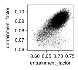
and exp_name = "ent-det-tked-tkee-stab-calibration" or one obtains

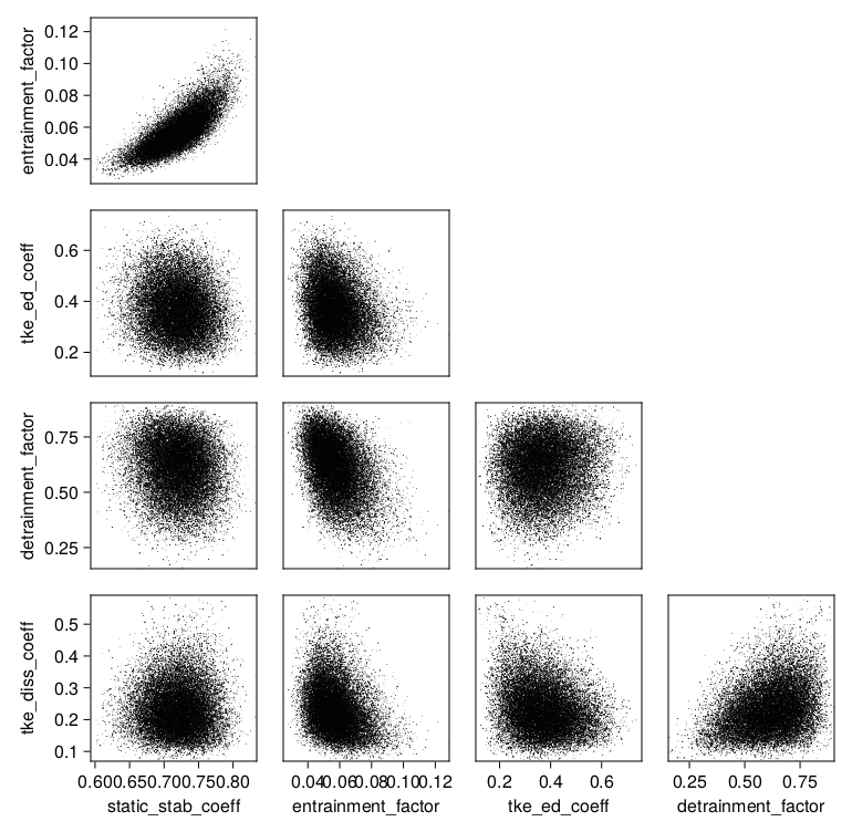
The posterior samples can also be investigated directly. They are stored as a ParameterDistribution-type Samples object. One can load this and extract an array of parameters with:

# input:
# path to posterior.jld2: posterior_filepath (string)

using CalibrateEmulateSample.ParameterDistribution
posterior = load(posterior_filepath)["posterior"]
posterior_samples = vcat([get_distribution(posterior)[name] for name in get_name(posterior)]...) # samples are columns

To transform these samples into physical parameter space use the following:

transformed_posterior_samples =
mapslices(x -> transform_unconstrained_to_constrained(posterior, x), posterior_samples, dims = 1)

Computational vs Physical space

The computational $\theta$-space are the parameters on which the algorithms act. Statistics (e.g. mean/covariance) are most meaningful when taken in this space. The physical $\phi$-space is a (nonlinear) transformation of the computational space to apply parameter constraints. To pass parameter values back into the forward model, one must transform them. Full details and examples can be found here