Regression of $\mathbb{R}^2 \to \mathbb{R}^2$ smooth function
The full code is found in the examples/Emulator/ directory of the github repository
In this example, we assess directly the performance of our machine learning emulators. The task is to learn the function:
\[G\colon [0,2\pi]^2 \to \mathbb{R}^2, G(x_1,x_2) = (\sin(x_1) + \cos(x_2), \sin(x_1) - \cos(x_2)) \]
observed at 150 points, subject to additive (and possibly correlated) Gaussian noise $N(0,\Sigma)$.
We have several different emulator configurations in this example that the user can play around with. The goal of this example is to predict the function (i.e. posterior mean) and uncertainty (i.e posterior pointwise variance) on a $200\times200$ grid providing a mean square error between emulated and true function and with plot_flag = true we also save several plots.
We will term scalar-output Gaussin process emulator as "GP", scalar-output random feature emulator as "scalar RF", and vector-output random feature emulator as "vector RF" henceforth.
Walkthrough of the code
We first import some standard packages
using Random
using StableRNGs
using Distributions
using Statistics
using LinearAlgebra
and relevant CES packages needed to define the emulators, packages and kernel structures
using CalibrateEmulateSample.Emulators
# Contains `Emulator`, `GaussianProcess`, `ScalarRandomFeatureInterface`, `VectorRandomFeatureInterface`
# `GPJL`, `SKLJL`, `SeparablKernel`, `NonSeparableKernel`, `OneDimFactor`, `LowRankFactor`, `DiagonalFactor`
using CalibrateEmulateSample.DataContainers # Contains `PairedDataContainer`
To play with the hyperparameter optimization of RF, the optimizer options sometimes require EnsembleKalmanProcesses.jl structures, so we load this too
using CalibrateEmulateSample.EnsembleKalmanProcesses # Contains `DataMisfitController`We have 9 cases that the user can toggle or customize
cases = [
    "gp-skljl",
    "gp-gpjl", # Very slow prediction...
    "rf-scalar",
    "rf-svd-diag",
    "rf-svd-nondiag",
    "rf-nosvd-diag",
    "rf-nosvd-nondiag",
    "rf-svd-nonsep",
    "rf-nosvd-nonsep",
]
The first two are for GP with either ScikitLearn.jl or GaussianProcesses.jl interface. The third is for the scalar RF interface, which most closely follows exactly replacing a GP. The rest are examples of vector RF with different types of data processing, (svd = same processing as scalar RF, nosvd = unprocessed) and different RF kernel structures in the output space of increasing complexity/flexibility (diag = Separable diagonal, nondiag = Separable nondiagonal, nonsep = nonseparable nondiagonal).
We set up the learning problem specification, defining input and output dimensions, and number of data to train on, and the function g and the perturbed samples y with correlated additive noise
n = 150  # number of training points
p = 2   # input dim
d = 2   # output dim
X = 2.0 * π * rand(p, n)
# G(x1, x2)
g1x = sin.(X[1, :]) .+ cos.(X[2, :])
g2x = sin.(X[1, :]) .- cos.(X[2, :])
gx = zeros(2, n)
gx[1, :] = g1x
gx[2, :] = g2x
# Add noise η
μ = zeros(d)
Σ = 0.1 * [[0.8, 0.1] [0.1, 0.5]] # d x d
noise_samples = rand(MvNormal(μ, Σ), n)
# y = G(x) + η
Y = gx .+ noise_samples
We then enter this in a paired data container, which gives a standard of how the data will be read
iopairs = PairedDataContainer(X, Y, data_are_columns = true)We define some common settings for all emulators, e.g. the number of random features to use, and some hyperparameter optimizer options
# common Gaussian feature setup
pred_type = YType()

# common random feature setup
n_features = 150
optimizer_options = Dict("n_iteration" => 10, "scheduler" => DataMisfitController(on_terminate = "continue"))
nugget = 1e-12
We then build the emulators. An example for GP (gp-skljl)
# use scikit learn
gppackage = SKLJL()
# build a GP that learns an additional white noise kernel (along with the default RBF kernel)
gaussian_process = GaussianProcess(gppackage, noise_learn = true)
# the data processing normalizes input data, and decorrelates output data with information from Σ
emulator = Emulator(gaussian_process, iopairs, obs_noise_cov = Σ, normalize_inputs = true)
An example for scalar RF (rf-scalar)
# build a scalar RF with a rank-2 kernel in input space (placeholder 1D kernel in output space) and use the optimizer options during training
srfi = ScalarRandomFeatureInterface(
    n_features,
    p,
    kernel_structure = SeparableKernel(LowRankFactor(2, nugget), OneDimFactor()),
    optimizer_options = optimizer_options,
)
# the data processing normalizes input data, and decorrelates output data with information from Σ
emulator = Emulator(srfi, iopairs, obs_noise_cov = Σ, normalize_inputs = true)
An example for vector RF (rf-nosvd-nonsep)
# build a vector RF with a rank-4 nonseparable kernel and use the optimizer options during training
vrfi = VectorRandomFeatureInterface(
    n_features,
    p,
    d, # additionally provide the output dimensions size
    kernel_structure = NonseparableKernel(LowRankFactor(4, nugget)),
    optimizer_options = optimizer_options,
)
# the data processing normalizes input data, and does not decorrelate outputs
emulator = Emulator(vrfi, iopairs, obs_noise_cov = Σ, normalize_inputs = true, decorrelate = false)
For RF and some GP packages, the training occurs during construction of the Emulator, however sometimes one must call an optimize step afterwards
optimize_hyperparameters!(emulator)Validation and Plots
We create an evaluation grid for our models, in the right shape:
n_pts = 200
x1 = range(0.0, stop = 2 * π, length = n_pts)
x2 = range(0.0, stop = 2 * π, length = n_pts)
X1, X2 = meshgrid(x1, x2)
inputs = permutedims(hcat(X1[:], X2[:]), (2, 1))
We predict using the emulators at the new inputs, and transform_to_real inverts the data processing back to physical values
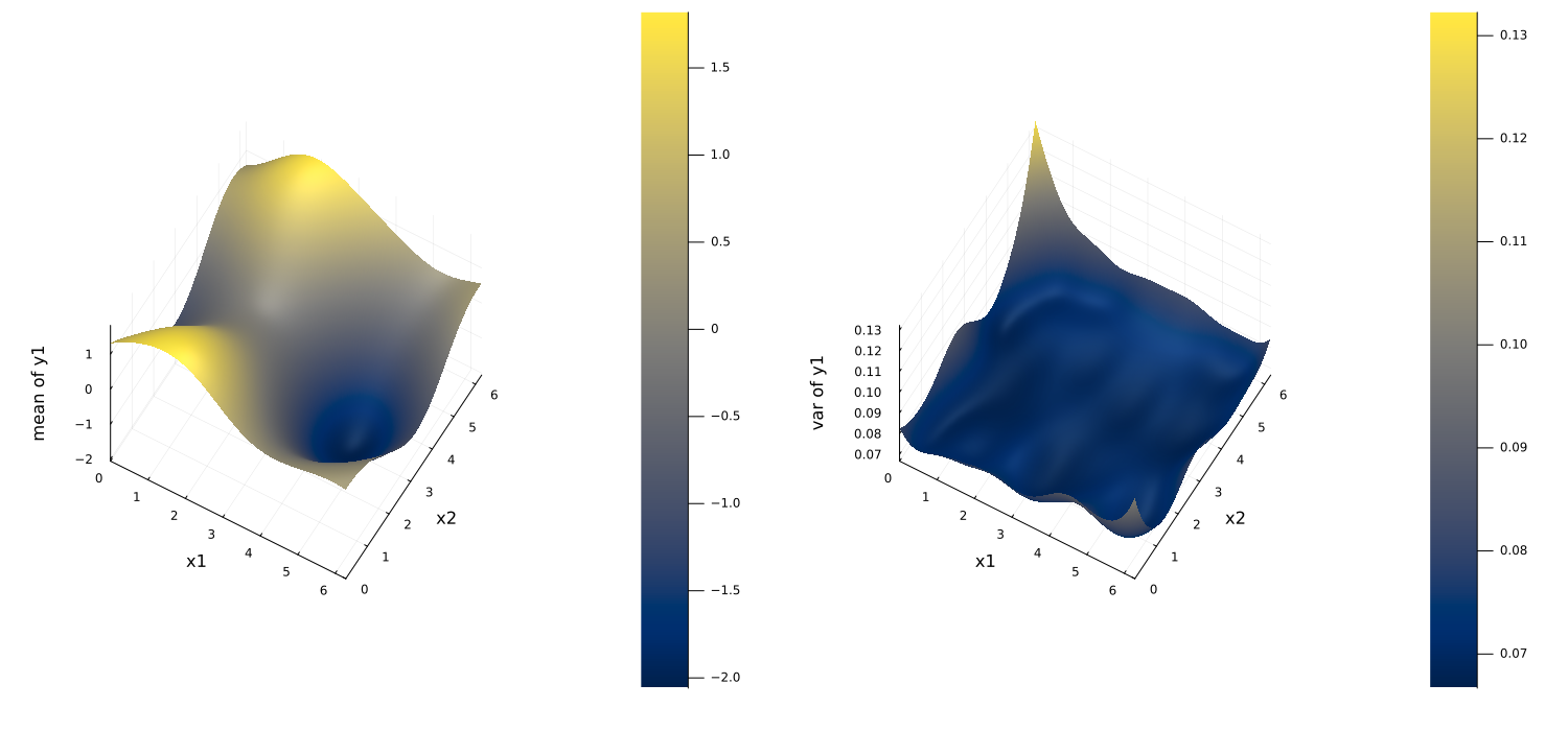
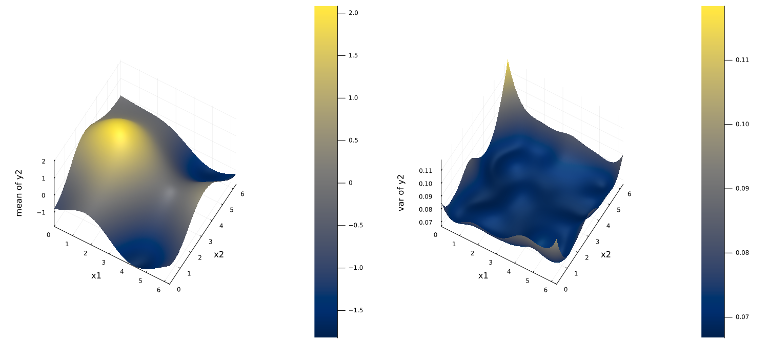
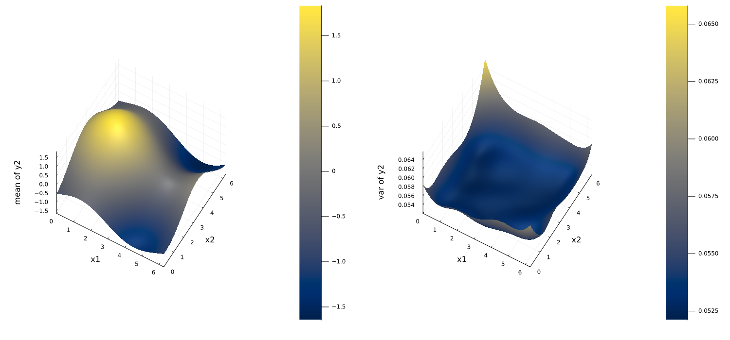
em_mean, em_cov = predict(emulator, inputs, transform_to_real = true)We then plot the predicted mean and pointwise variances, and calculate the errors from the three highlighted cases:
Gaussian Process Emulator (Sci-kit learn: gp-skljl)
L^2 error of mean and latent truth:0.0008042391077774167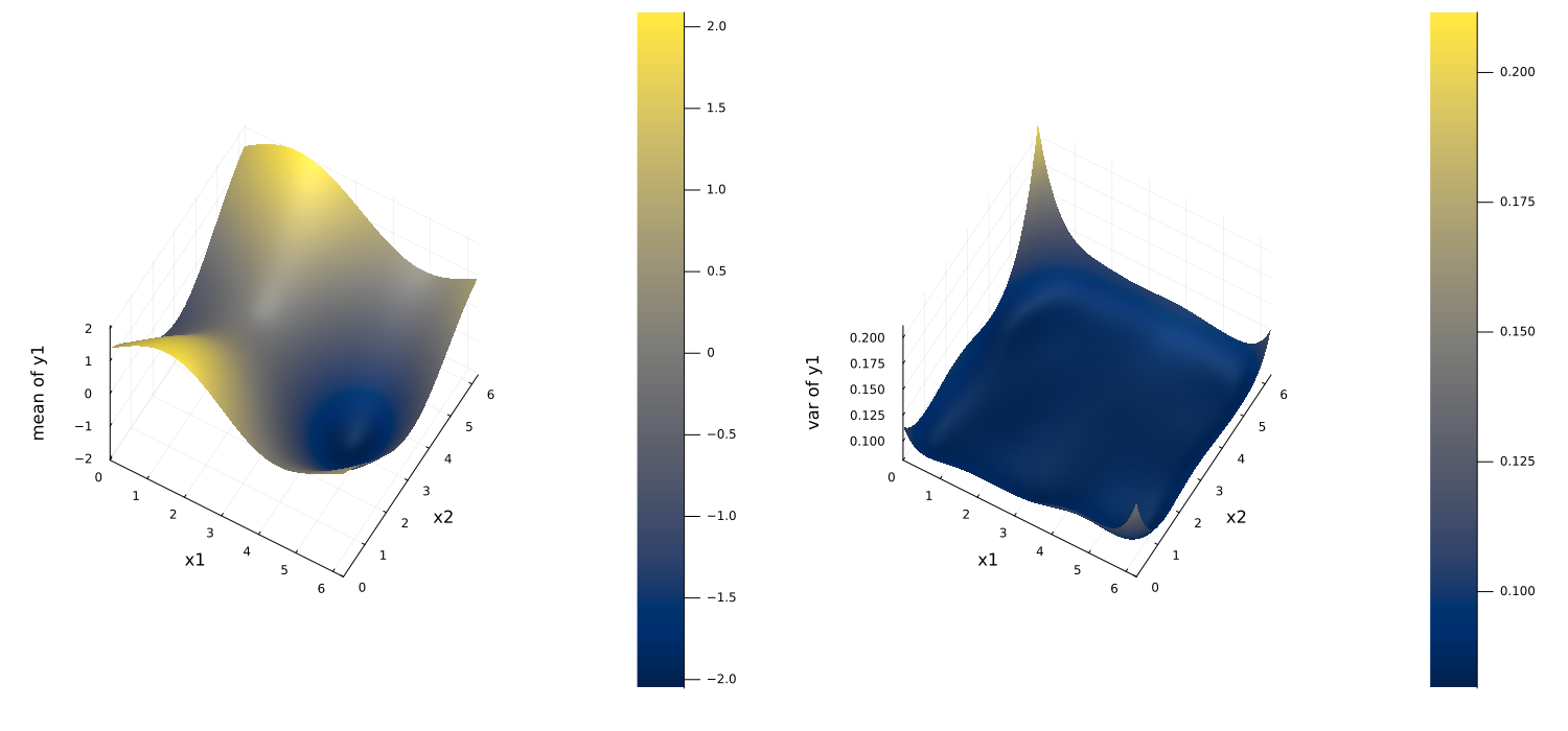
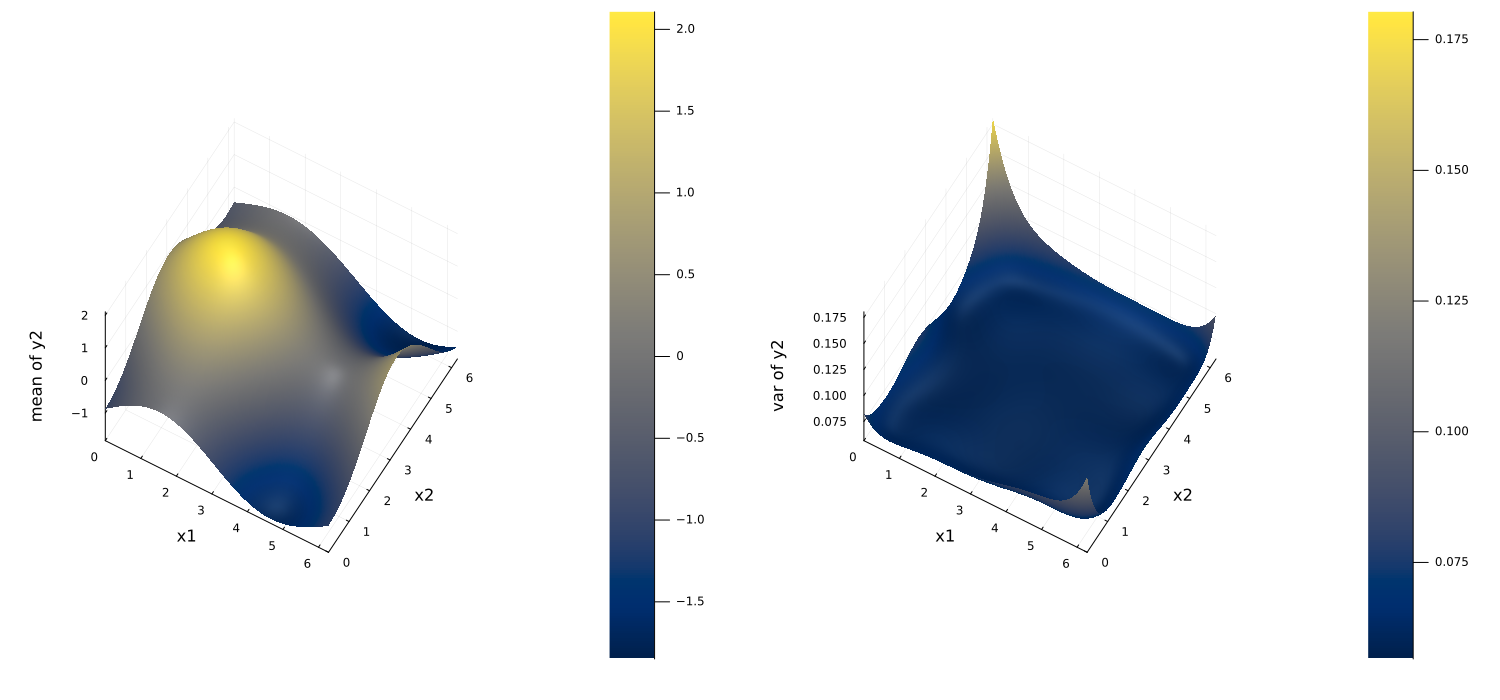
Random Feature Emulator (rf-scalar)
L^2 error of mean and latent truth:0.0012253119679379056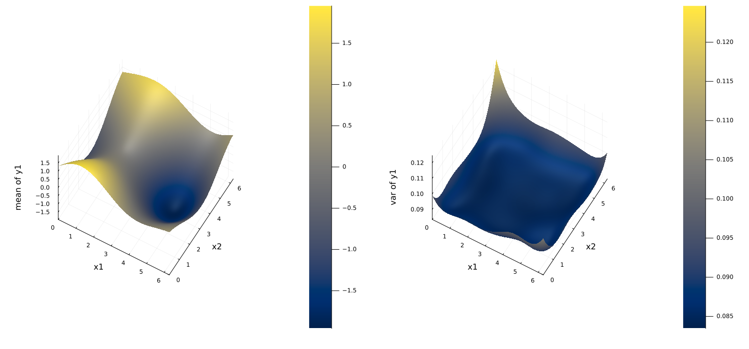
Random Feature Emulator (vector: rf-nosvd-nonsep)
L^2 error of mean and latent truth:0.0011094292509180393