Lorenz 96 example

The Lorenz 96 (hereafter L96) example is a toy-problem for the application of the CalibrateEmulateSample.jl optimization and approximate uncertainty quantification methodologies. Here is L96 with additional periodic-in-time forcing, we try to determine parameters (sinusoidal amplitude and stationary component of the forcing) from some output statistics. The standard L96 equations are implemented with an additional forcing term with time dependence. The output statistics which are used for learning are the finite time-averaged variances.

The standard single-scale L96 equations are implemented. The Lorenz 96 system (Lorenz, 1996) is given by

\[\frac{d x_i}{d t} = (x_{i+1} - x_{i-2}) x_{i-1} - x_i + F,\]

with $i$ indicating the index of the given longitude. The number of longitudes is given by $N$. The boundary conditions are given by

\[x_{-1} = x_{N-1}, \ x_0 = x_N, \ x_{N+1} = x_1.\]

The time scaling is such that the characteristic time is 5 days (Lorenz, 1996). For very small values of $F$, the solutions $x_i$ decay to $F$ after the initial transient feature. For moderate values of $F$, the solutions are periodic, and for larger values of $F$, the system is chaotic. The solution variance is a function of the forcing magnitude. Variations in the base state as a function of time can be imposed through a time-dependent forcing term $F(t)$.

A temporal forcing term is defined

\[F = F_s + A \sin(\omega t),\]

with steady-state forcing $F_s$, transient forcing amplitude $A$, and transient forcing frequency $\omega$. The total forcing $F$ must be within the chaotic regime of L96 for all time given the prescribed $N$.

The L96 dynamics are solved with RK4 integration.

Structure

The example is structured with two distinct components: 1) L96 dynamical system solver; 2) calibrate-emulate sample code. Each of these are described below.

The forward mapping from input parameters to output statistics of the L96 system is solved using the GModel.jl code, which runs the L96 model across different input parameters $\theta$. The source code for the L96 system solution is within the GModel_common.jl code.

The Calibrate code is located in calibrate.jl which provides the functionality to run the L96 dynamical system (within the GModel.jl code), extract time-averaged statistics from the L96 states, and use the time-average statistics for calibration. While this example description is self-contained, there is an additional description of the use of EnsembleKalmanProcesses.jl for the L96 example that is accessible here.

The Emulate-Sample code is located in emulate_sample.jl which provides the functionality to use the input-output pairs from the Calibrate stage for emulation and sampling (uncertainty quantification). The emulate_sample.jl code relies on outputs from the calibrate.jl code

Walkthrough of the code

This walkthrough covers calibrate-emulate-sample for the L96 problem defined above. The goal is to learn parameters F_s and A based on the time averaged statistics in a perfect model setting. This document focuses on the emulate-sample (emulate_sample.jl) stages, but discussion of the calibration stage calibrate.jl are made when necessary. This code relies on data generated by first running calibrate.jl. A detailed walkthrough of the calibration stage of CES for the L96 example is available here.

Inputs

First, we load standard packages

# Import modules
using Distributions  # probability distributions and associated functions
using LinearAlgebra
using StatsPlots
using Plots
using Random
using JLD2

Then, we load CalibrateEmulateSample.jl packages

# CES 
using CalibrateEmulateSample.Emulators
using CalibrateEmulateSample.MarkovChainMonteCarlo
using CalibrateEmulateSample.Utilities
using CalibrateEmulateSample.EnsembleKalmanProcesses
using CalibrateEmulateSample.ParameterDistributions
using CalibrateEmulateSample.DataContainers
using CalibrateEmulateSample.Observations

The first input settings define which input-output pairs to use for training the emulator. The Calibrate stage (run using calibrate.jl) generates parameter-to-data pairs by running the L96 system using an iterative optimization approach (EnsembleKalmanProcess.jl). So we first define which iterations we would like to use data from for our emulator training

min_iter = 1
max_iter = 5 # number of EKP iterations to use data from is at most this

The second input settings define the Lorenz dynamics. The emulate_sample.jl code does not actually run the L96 system, it only uses L96 system runs from the calibrate.jl stage to train an emulator and to perform sampling. Therefore, the settings governing the L96 dynamics are fully defined in calibrate.jl and can be modified as necessary. The rest of the input settings in this section are defined in calibrate.jl.

F_true = 8.0 # Mean F
A_true = 2.5 # Transient F amplitude
ω_true = 2.0 * π / (360.0 / τc) # Frequency of the transient F (non-dim)
params_true = [F_true, A_true]
param_names = ["F", "A"]

The use of the transient forcing term is with the flag, dynamics. Stationary forcing is dynamics=1 ($A=0$) and transient forcing is used with dynamics=2 ($A\neq0$). The system with $N$ longitudes is solved over time horizon t_start to Tfit at fixed time step dt.

N = 36
dt = 1/64
t_start = 100
# Characteristic time scale
τc = 5.0 # days, prescribed by the L96 problem
# This has to be less than 360 and 360 must be divisible by Ts_days
Ts_days = 30.0 # Integration length in days (will be made non-dimensional later)
# Integration length
Tfit = Ts_days / τc

The states are integrated over time Ts_days to construct the time averaged statistics for use by the Ensemble Kalman Process calibration. The specification of the statistics to be gathered from the states are provided by stats_type.

We implement (biased) priors as follows

prior_means = [F_true + 1.0, A_true + 0.5]
prior_stds = [2.0, 0.5 * A_true]
# constrained_gaussian("name", desired_mean, desired_std, lower_bd, upper_bd)
prior_F = constrained_gaussian(param_names[1], prior_means[1], prior_stds[1], 0, Inf)
prior_A = constrained_gaussian(param_names[2], prior_means[2], prior_stds[2], 0, Inf)
priors = combine_distributions([prior_F, prior_A])

We use the recommended [constrained_gaussian] to add the desired scale and bounds to the prior distribution, in particular we place lower bounds to preserve positivity.

The priors can be plotted directly using plot(priors), as seen below in the example code from calibrate.jl

# Plot the prior distribution
p = plot(priors, title = "prior")
plot!(p.subplots[1], [F_true], seriestype = "vline", w = 1.5, c = :steelblue, ls = :dash, xlabel = "F") # vline on top histogram
plot!(p.subplots[2], [A_true], seriestype = "vline", w = 1.5, c = :steelblue, ls = :dash, xlabel = "A") # vline on top histogram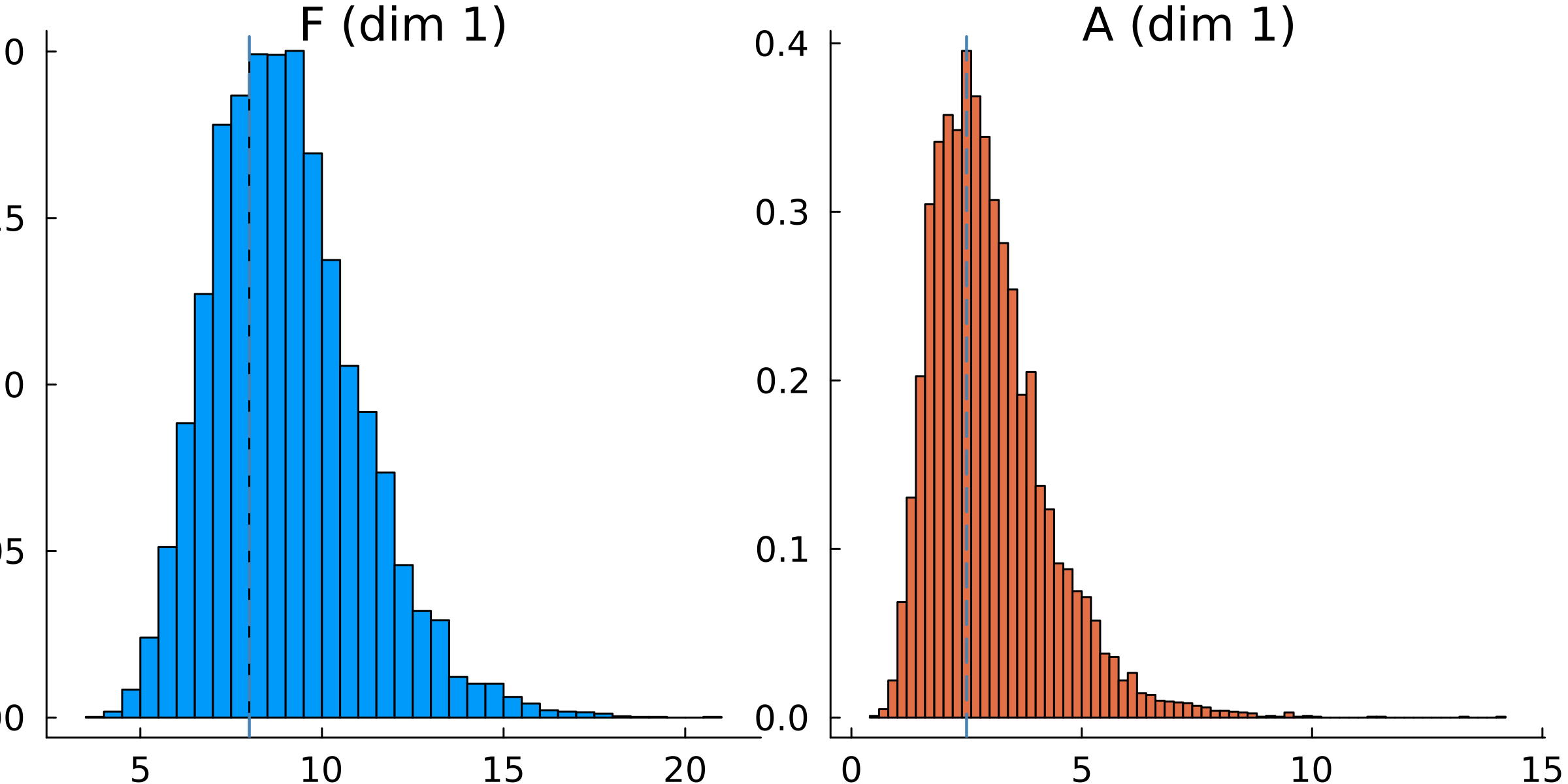

The observational noise can be generated using the L96 system or prescribed, as specified by var_prescribe. var_prescribe==false The observational noise is constructed by generating independent instantiations of the L96 statistics of interest at the true parameters for different initial conditions. The empirical covariance matrix is constructed.

var_prescribe==true The observational noise is prescribed as a Gaussian distribution with prescribed mean and variance.

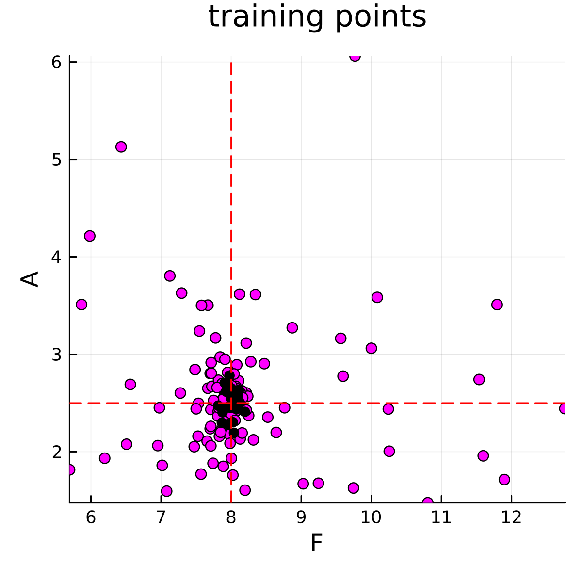
Calibrate

The calibration stage must be run before the emulate-sample stages. The calibration stage is run using calibrate.jl. This code will generate parameter-data pairs that will be used to train the emulator. The parameter-data pairs are visualized below

Emulate

Having run the calibrate.jl code to generate input-output pairs from parameters to data using EnsembleKalmanProcesses.jl, we will now run the Emulate and Sample stages (emulate_sample.jl). First, we need to define which machine learning model we will use for the emulation. We have 8 cases that the user can toggle or customize

cases = [
        "GP", # diagonalize, train scalar GP, assume diag inputs
        "RF-scalar-diagin", # diagonalize, train scalar RF, assume diag inputs (most comparable to GP)
        "RF-scalar", # diagonalize, train scalar RF, do not asume diag inputs
        "RF-vector-svd-diag",
        "RF-vector-svd-nondiag",
        "RF-vector-nosvd-diag",
        "RF-vector-nosvd-nondiag",
        "RF-vector-svd-nonsep",
]

The first is for GP with GaussianProcesses.jl interface. The next two are for the scalar RF interface, which most closely follows exactly replacing a GP. The rest are examples of vector RF with different types of data processing, (svd = same processing as scalar RF, nosvd = unprocessed) and different RF kernel structures in the output space of increasing complexity/flexibility (diag = Separable diagonal, nondiag = Separable nondiagonal, nonsep = nonseparable nondiagonal).

The example then loads the relevant training data that was constructed in the calibrate.jl call.

# loading relevant data
homedir = pwd()
println(homedir)
figure_save_directory = joinpath(homedir, "output/")
data_save_directory = joinpath(homedir, "output/")
data_save_file = joinpath(data_save_directory, "calibrate_results.jld2")
ekiobj = load(data_save_file)["eki"]
priors = load(data_save_file)["priors"]
truth_sample_mean = load(data_save_file)["truth_sample_mean"]
truth_sample = load(data_save_file)["truth_sample"]
truth_params_constrained = load(data_save_file)["truth_input_constrained"] #true parameters in constrained space
truth_params = transform_constrained_to_unconstrained(priors, truth_params_constrained)
Γy = ekiobj.obs_noise_cov

We then set up the structure of the emulator. An example for GP (GP)

gppackage = Emulators.GPJL()
pred_type = Emulators.YType()
mlt = GaussianProcess(
    gppackage;
    kernel = nothing, # use default squared exponential kernel
    prediction_type = pred_type,
    noise_learn = false,
)

which calls GaussianProcess.jl. In this L96 example, since we focus on learning $F_s$ and $A$, we do not need to explicitly learn the noise, so noise_learn = false.

An example for scalar RF (RF-scalar)

n_features = 100
kernel_structure = SeparableKernel(LowRankFactor(2, nugget), OneDimFactor())
mlt = ScalarRandomFeatureInterface(
    n_features,
    n_params,
    rng = rng,
    kernel_structure = kernel_structure,
    optimizer_options = overrides,
)

Optimizer options for ScalarRandomFeature.jl are provided throough overrides

overrides = Dict(
            "verbose" => true,
            "scheduler" => DataMisfitController(terminate_at = 100.0),
            "cov_sample_multiplier" => 1.0,
            "n_iteration" => 20,
        )
# we do not want termination, as our priors have relatively little interpretation

We then build the emulator with the parameters as defined above

emulator = Emulator(
            mlt,
            input_output_pairs;
            obs_noise_cov = Γy,
            normalize_inputs = normalized,
            standardize_outputs = standardize,
            standardize_outputs_factors = norm_factor,
            retained_svd_frac = retained_svd_frac,
            decorrelate = decorrelate,
        )

For RF and some GP packages, the training occurs during construction of the Emulator, however sometimes one must call an optimize step afterwards

optimize_hyperparameters!(emulator)

The emulator is checked for accuracy by evaluating its predictions on the true parameters

# Check how well the Gaussian Process regression predicts on the
# true parameters
y_mean, y_var = Emulators.predict(emulator, reshape(truth_params, :, 1), transform_to_real = true)
y_mean_test, y_var_test = Emulators.predict(emulator, get_inputs(input_output_pairs_test), transform_to_real = true)

println("ML prediction on true parameters: ")
println(vec(y_mean))
println("true data: ")
println(truth_sample) # what was used as truth
println(" ML predicted standard deviation")
println(sqrt.(diag(y_var[1], 0)))
println("ML MSE (truth): ")
println(mean((truth_sample - vec(y_mean)) .^ 2))
println("ML MSE (next ensemble): ")
println(mean((get_outputs(input_output_pairs_test) - y_mean_test) .^ 2))

Sample

Now the emulator is constructed and validated, so we next focus on the MCMC sampling. First, we run a short chain ($2,000$ steps) to determine the step size

# First lets run a short chain to determine a good step size
mcmc = MCMCWrapper(RWMHSampling(), truth_sample, priors, emulator; init_params = u0)
new_step = optimize_stepsize(mcmc; init_stepsize = 0.1, N = 2000, discard_initial = 0)

The step size has been determined, so now we run the full MCMC ($100,000$ steps where the first $2,000$ are discarded)

# Now begin the actual MCMC
println("Begin MCMC - with step size ", new_step)
chain = MarkovChainMonteCarlo.sample(mcmc, 100_000; stepsize = new_step, discard_initial = 2_000)

And we finish by extracting the posterior samples

posterior = MarkovChainMonteCarlo.get_posterior(mcmc, chain)

And evaluate the results with these printed statements

post_mean = mean(posterior)
post_cov = cov(posterior)
println("post_mean")
println(post_mean)
println("post_cov")
println(post_cov)
println("D util")
println(det(inv(post_cov)))
println(" ")

Running the Example and Postprocessing

First, the calibrate code must be executed, which will perform the calibration step and, generating input-output pairs of the parameter to data mapping. Then, the emulate-sample code is run, which will load the input-ouput pairs that were generated in the calibration step.

Calibrate

The L96 parameter calibration can be run using julia --project calibrate.jl

The output will provide the estimated parameters in the constrained ϕ-space. The priors are required in the get-method to apply these constraints.

Printed output:

# EKI results: Has the ensemble collapsed toward the truth?
println("True parameters: ")
println(params_true)
println("\nEKI results:")
println(get_ϕ_mean_final(priors, ekiobj))

The parameters and forward model outputs will be saved in parameter_storage.jld2 and data_storage.jld2, respectively. The data will be saved in the directory output. A scatter plot animation of the ensemble convergence to the true parameters is saved in the directory output. These points represent the training points that are used for the emulator.

Emulate-sample

The L96 parameter estimation can be run using julia --project emulate_sample.jl

The output will provide the estimated posterior distribution over the parameters. The emulate-sample code will run for several choices in the machine learning model that is used for the emulation stage, inclding Gaussian Process regression and RF, and using singular value data decorrelation or not.

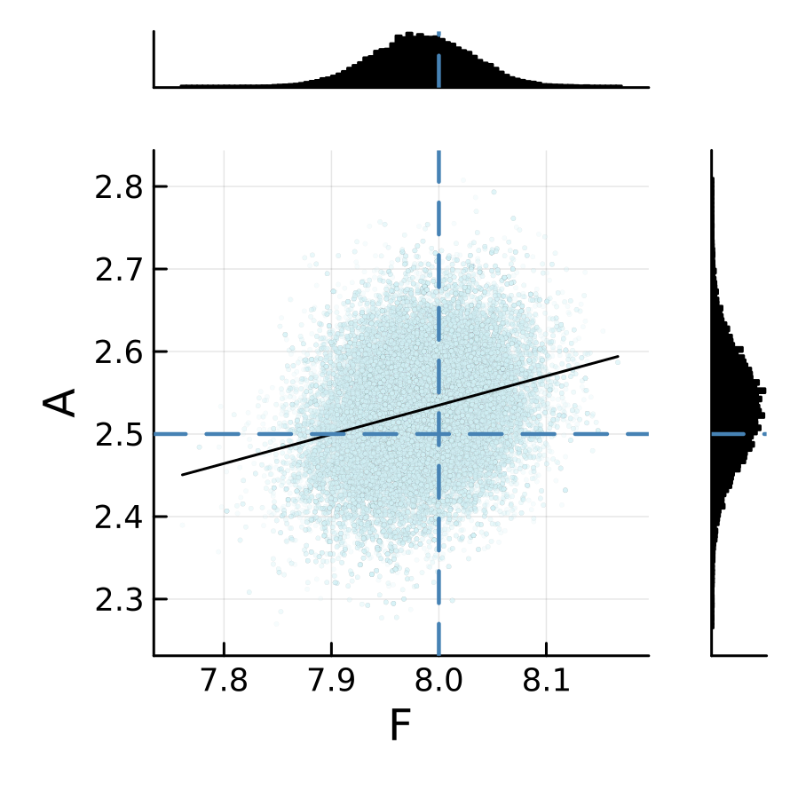
The sampling results from two emulators are shown below. We can see that the posterior is relatively insensitive to the choice of the machine learning emulation tool in this L96 example.

L96 CES example case: GP regression emulator (case="GP")

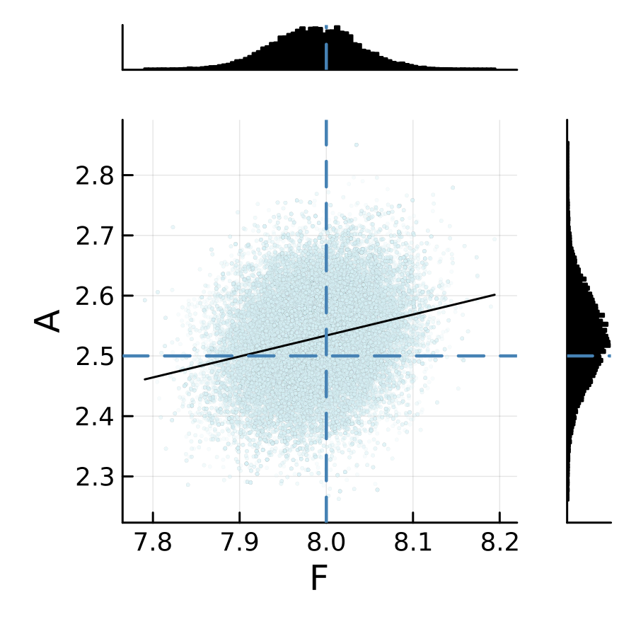
L96 CES example case: RF scalar emulator (case="RF-scalar")