Perfect Model Site-Level Calibration Tutorial

This tutorial demonstrates how to perform a perfect model calibration experiment using ClimaLand. In a perfect model experiment, we generate synthetic observations from our model with known parameters, then use ensemble Kalman inversion to recover those parameters. This approach allows us to evaluate the calibration method without the influence of model structural errors.

In this tutorial we will calibrate the Vcmax25 parameter using latent heat flux observations from the FLUXNET site (US-MOz).

Overview

The tutorial covers:

1. Setting up a land surface model for a FLUXNET site (US-MOz)
2. Creating a synthetic observation dataset
3. Implementing Ensemble Kalman Inversion
4. Analyzing the calibration results

Setup and Imports

Load all the necessary packages for land surface modeling, diagnostics, plotting, and ensemble methods:

using ClimaLand
using ClimaLand.Domains: Column
using ClimaLand.Canopy
using ClimaLand.Simulations
import ClimaLand.FluxnetSimulations as FluxnetSimulations
import ClimaLand.Parameters as LP
import ClimaLand.LandSimVis as LandSimVis
import ClimaDiagnostics
import EnsembleKalmanProcesses as EKP
import EnsembleKalmanProcesses.ParameterDistributions as PD
using CairoMakie
CairoMakie.activate!()
using Statistics
using Logging
import Random
using Dates
using ClimaAnalysis, GeoMakie, Printf

Configuration and Site Setup

Configure the experiment parameters and set up the FLUXNET site (US-MOz) with its specific location, time settings, and atmospheric conditions.

Set random seed for reproducibility and floating point precision

rng_seed = 1234
rng = Random.MersenneTwister(rng_seed)
const FT = Float32

Float32

Initialize land parameters and site configuration.

toml_dict = LP.create_toml_dict(FT)
site_ID = "US-MOz"
site_ID_val = FluxnetSimulations.replace_hyphen(site_ID)

:US_MOz

Get site-specific information: location coordinates, time offset, and sensor height.

(; time_offset, lat, long) =
    FluxnetSimulations.get_location(FT, Val(site_ID_val))
(; atmos_h) = FluxnetSimulations.get_fluxtower_height(FT, Val(site_ID_val))

(atmos_h = 32.0f0,)

Get maximum simulation start and end dates

(start_date, stop_date) =
    FluxnetSimulations.get_data_dates(site_ID, time_offset)
stop_date = DateTime(2010, 4, 1, 6, 30)  # Set the stop date manually
Δt = 450.0  # seconds

450.0

Domain and Forcing Setup

Create the computational domain and load the necessary forcing data for the land surface model.

Create a column domain representing a 2-meter deep soil column with 10 vertical layers.

zmin = FT(-2)  # 2m depth
zmax = FT(0)   # surface
domain = Column(; zlim = (zmin, zmax), nelements = 10, longlat = (long, lat));

Load prescribed atmospheric and radiative forcing from FLUXNET data

forcing = FluxnetSimulations.prescribed_forcing_fluxnet(
    site_ID,
    lat,
    long,
    time_offset,
    atmos_h,
    start_date,
    toml_dict,
    FT,
);

Model Setup

Create an integrated land model that couples canopy, snow, soil, and soil CO2 components. This comprehensive model allows us to simulate the full land surface system and its interactions.

function model(Vcmax25)
    #md # Get Leaf Area Index (LAI) data from MODIS satellite observations.
    LAI = ClimaLand.Canopy.prescribed_lai_modis(
        domain.space.surface,
        start_date,
        stop_date,
    )
    Vcmax25 = FT(Vcmax25)

    #md # Set up ground conditions and define which components to simulate prognostically
    ground = ClimaLand.PrognosticGroundConditions{FT}()
    prognostic_land_components = (:canopy, :snow, :soil, :soilco2)

    #md # Prepare canopy domain and forcing
    canopy_domain = ClimaLand.Domains.obtain_surface_domain(domain)
    canopy_forcing = (; forcing.atmos, forcing.radiation, ground)

    #md # Set up photosynthesis parameters using the Farquhar model
    photosyn_defaults =
        Canopy.clm_photosynthesis_parameters(canopy_domain.space.surface)
    photosynthesis = Canopy.FarquharModel{FT}(
        canopy_domain,
        toml_dict;
        photosynthesis_parameters = (;
            fractional_c3 = photosyn_defaults.fractional_c3,
            Vcmax25,
        ),
    )

    conductance = Canopy.MedlynConductanceModel{FT}(
        canopy_domain,
        toml_dict;
        g1 = FT(141),
    )

    #md # Create canopy model
    canopy = ClimaLand.Canopy.CanopyModel{FT}(
        canopy_domain,
        canopy_forcing,
        LAI,
        toml_dict;
        photosynthesis,
        prognostic_land_components,
        conductance,
    )

    #md # Create integrated land model
    land_model = LandModel{FT}(
        forcing,
        LAI,
        toml_dict,
        domain,
        Δt;
        prognostic_land_components,
        canopy,
    )

    #md # Set initial conditions from FLUXNET data
    set_ic! = FluxnetSimulations.make_set_fluxnet_initial_conditions(
        site_ID,
        start_date,
        time_offset,
        land_model,
    )

    #md # Configure diagnostics to output sensible and latent heat fluxes hourly
    output_vars = ["shf", "lhf"]
    diagnostics = ClimaLand.default_diagnostics(
        land_model,
        start_date;
        output_writer = ClimaDiagnostics.Writers.DictWriter(),
        output_vars,
        reduction_period = :hourly,
    )

    #md # Create and run the simulation
    simulation = Simulations.LandSimulation(
        start_date,
        stop_date,
        Δt,
        land_model;
        set_ic!,
        user_callbacks = (),
        diagnostics,
    )
    solve!(simulation)
    return simulation
end

model (generic function with 1 method)

Observation and Helper Functions

Define the observation function G that maps from parameter space to observation space, along with supporting functions for data processing:

This function runs the model and computes diurnal average of latent heat flux

function G(Vcmax25)
    simulation = model(Vcmax25)
    lhf = get_lhf(simulation)
    observation =
        Float64.(
            get_diurnal_average(
                lhf,
                simulation.start_date,
                simulation.start_date + Day(20),
            ),
        )
    return observation
end

G (generic function with 1 method)

Helper function: Extract latent heat flux from simulation diagnostics

function get_lhf(simulation)
    return ClimaLand.Diagnostics.diagnostic_as_vectors(
        simulation.diagnostics[1].output_writer,
        "lhf_1h_average",
    )
end

get_lhf (generic function with 1 method)

Helper function: Compute diurnal average of a variable

function get_diurnal_average(var, start_date, spinup_date)
    (times, data) = var
    model_dates = if times isa Vector{DateTime}
        times
    else
        Second.(getproperty.(times, :counter)) .+ start_date
    end
    spinup_idx = findfirst(spinup_date .<= model_dates)
    model_dates = model_dates[spinup_idx:end]
    data = data[spinup_idx:end]

    hour_of_day = Hour.(model_dates)
    mean_by_hour = [mean(data[hour_of_day .== Hour(i)]) for i in 0:23]
    return mean_by_hour
end

get_diurnal_average (generic function with 1 method)

Perfect Model Experiment Setup

Since this is a perfect model experiment, we generate synthetic observations from our target parameter value. This parameter will be recovered by the calibration.

true_Vcmax25 = 0.0001 # [mol m-2 s-1]
observations = G(true_Vcmax25)

24-element Vector{Float64}:
 61.74391555786133
 15.626395225524902
  6.621608734130859
  3.664515495300293
 18.45545768737793
  7.634608745574951
  4.12026309967041
 12.24223518371582
  6.840919017791748
  4.427279949188232
  8.953359603881836
  5.7875800132751465
  4.099796295166016
  4.910253047943115
  3.596738815307617
  2.7912445068359375
 29.37281036376953
 33.56330490112305
 34.76032638549805
 54.56296920776367
 60.1796875
 69.0430908203125
 57.0079231262207
 58.907901763916016

Define observation noise covariance for the ensemble Kalman process. A flat covariance matrix is used here for simplicity.

noise_covariance = 0.05 * EKP.I

LinearAlgebra.UniformScaling{Float64}
0.05*I

Prior Distribution and Calibration Configuration

Set up the prior distribution for the parameter and configure the ensemble Kalman inversion:

Constrained Gaussian prior for Vcmax25 with bounds [0, 2e-3]

prior = PD.constrained_gaussian("Vcmax25", 1e-3, 5e-4, 0, 2e-3)

ParameterDistribution with 1 entry
  'Vcmax25': Parameterized (Normal) [1 constraint]

Set the ensemble size and number of iterations

ensemble_size = 10
N_iterations = 3

3

Ensemble Kalman Inversion

Initialize and run the ensemble Kalman process:

Sample the initial parameter ensemble from the prior distribution

initial_ensemble = EKP.construct_initial_ensemble(rng, prior, ensemble_size)

ensemble_kalman_process = EKP.EnsembleKalmanProcess(
    initial_ensemble,
    observations,
    noise_covariance,
    EKP.Inversion();
    scheduler = EKP.DataMisfitController(
        terminate_at = Inf,
        on_terminate = "continue",
    ),
    rng,
)

EnsembleKalmanProcess
  process    : Inversion
  N_ens      : 10
  N_par      : 1
  n_iter     : 0
  scheduler  : DataMisfitController
  accelerator: NesterovAccelerator

Run the ensemble of forward models to iteratively update the parameter ensemble

Logging.with_logger(SimpleLogger(devnull, Logging.Error)) do
    for i in 1:N_iterations
        println("Iteration $i")
        params_i = EKP.get_ϕ_final(prior, ensemble_kalman_process)
        G_ens = hcat([G(params_i[:, j]...) for j in 1:ensemble_size]...)
        EKP.update_ensemble!(ensemble_kalman_process, G_ens)
    end
end

Iteration 1
Iteration 2
Iteration 3

Results Analysis and Visualization

Get the mean of the final parameter ensemble:

EKP.get_ϕ_mean_final(prior, ensemble_kalman_process)

1-element Vector{Float64}:
 0.0015265986376921006

Now, let's analyze the calibration results by examining parameter evolution and comparing model outputs across iterations.

Plot the parameter ensemble evolution over iterations to visualize convergence:

dim_size = sum(length.(EKP.batch(prior)))
fig = CairoMakie.Figure(size = ((dim_size + 1) * 500, 500))

for i in 1:dim_size
    EKP.Visualize.plot_ϕ_over_iters(
        fig[1, i],
        ensemble_kalman_process,
        prior,
        i,
    )
end

EKP.Visualize.plot_error_over_iters(
    fig[1, dim_size + 1],
    ensemble_kalman_process,
)
CairoMakie.save("perfect_model_constrained_params_and_error.png", fig);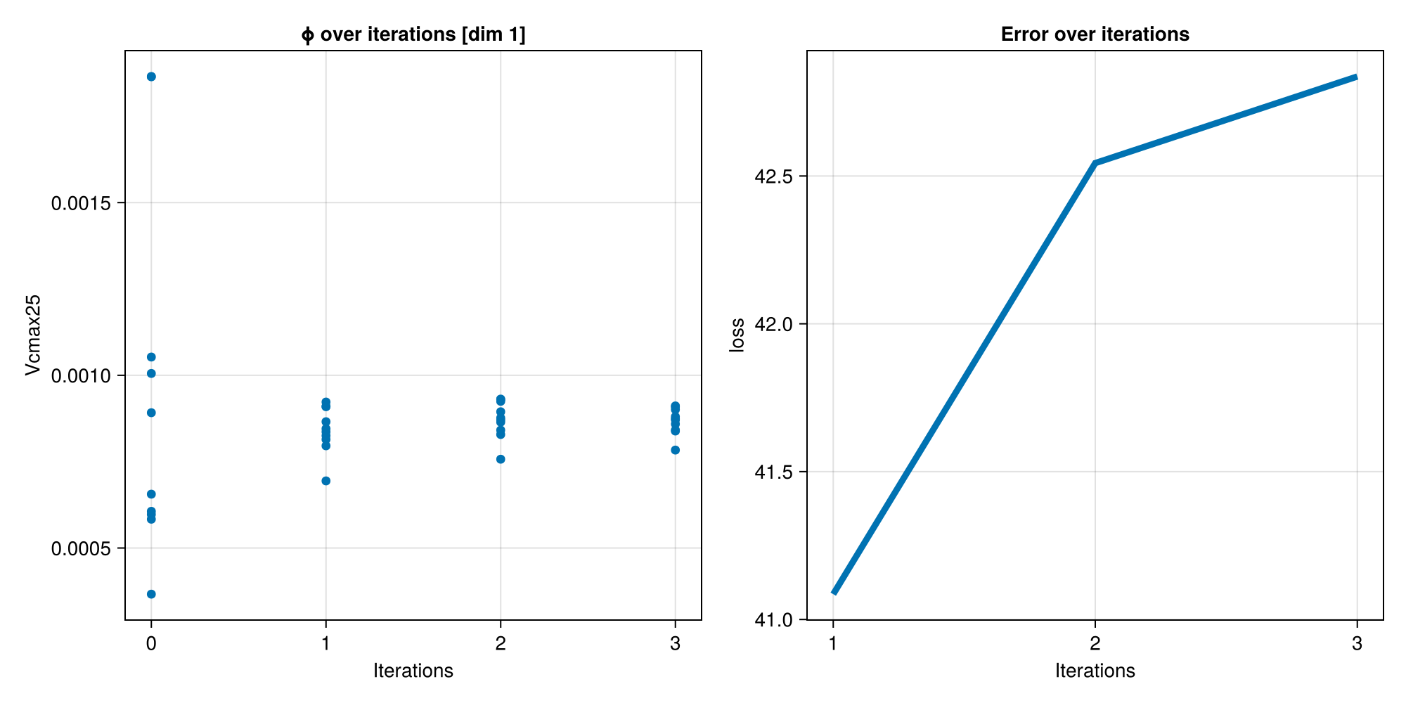

Compare the model output between the first and last iterations to assess improvement:

fig = CairoMakie.Figure(size = (900, 400))

first_G_ensemble = EKP.get_g(ensemble_kalman_process, 1)
last_iter = EKP.get_N_iterations(ensemble_kalman_process)
last_G_ensemble = EKP.get_g(ensemble_kalman_process, last_iter)
n_ens = EKP.get_N_ens(ensemble_kalman_process)

ax = Axis(
    fig[1, 1];
    title = "G ensemble: first vs last iteration (n = $(n_ens), iters 1 vs $(last_iter))",
    xlabel = "Observation index",
    ylabel = "G",
)

Makie.Axis with 0 plots:

Plot model output of first vs last iteration ensemble

for g in eachcol(first_G_ensemble)
    lines!(ax, 1:length(g), g; color = (:red, 0.6), linewidth = 1.5)
end

for g in eachcol(last_G_ensemble)
    lines!(ax, 1:length(g), g; color = (:blue, 0.6), linewidth = 1.5)
end

lines!(
    ax,
    1:length(observations),
    observations;
    color = (:black, 0.6),
    linewidth = 3,
)

axislegend(
    ax,
    [
        LineElement(color = :red, linewidth = 2),
        LineElement(color = :blue, linewidth = 2),
        LineElement(color = :black, linewidth = 4),
    ],
    ["First ensemble", "Last ensemble", "Observations"];
    position = :rb,
    framevisible = false,
)

CairoMakie.resize_to_layout!(fig)
CairoMakie.save("perfect_model_G_first_and_last.png", fig);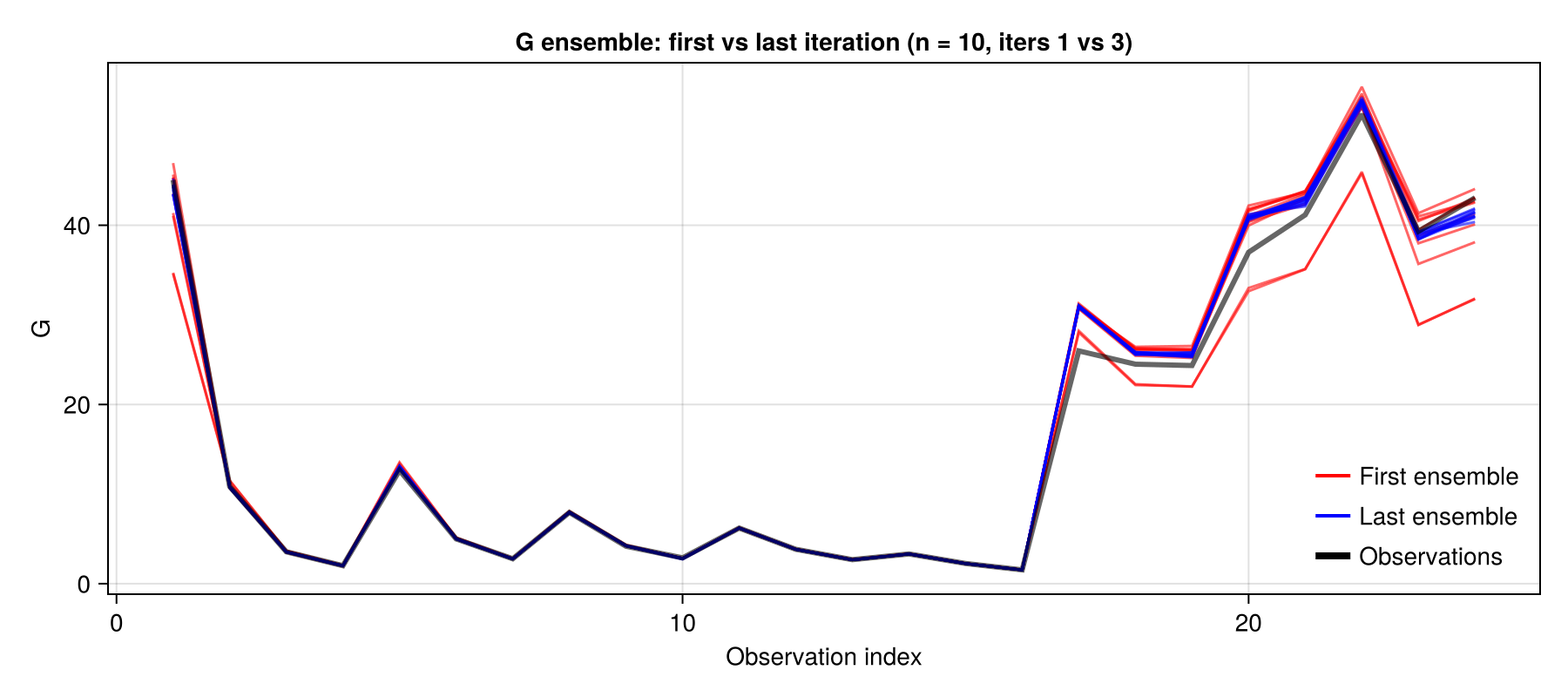

This page was generated using Literate.jl.