Eventually this will be a bare soil site experiment, showing how to set up the soil model in a column with prescribed forcing and comparing to data.

using CairoMakie
import ClimaTimeSteppers as CTS
using Thermodynamics

using ClimaCore
import ClimaParams as CP
using SurfaceFluxes
using StaticArrays
using Dates
using DelimitedFiles: readdlm

using ClimaLand
using ClimaLand.Domains: Column
using ClimaLand.Soil
import ClimaLand.Simulations: LandSimulation, solve!
import ClimaLand
import ClimaLand.Parameters as LP
import SurfaceFluxes.Parameters as SFP

FT = Float64;
toml_dict = LP.create_toml_dict(FT)
earth_param_set = LP.LandParameters(toml_dict)
thermo_params = LP.thermodynamic_parameters(earth_param_set);

start_date = DateTime(2005)
stop_date = start_date + Day(4)
dt = Float64(10)
SW_d = (t) -> 0
LW_d = (t) -> 270.0^4 * 5.67e-8
radiation = PrescribedRadiativeFluxes(
    FT,
    TimeVaryingInput(SW_d),
    TimeVaryingInput(LW_d),
    start_date,
);

Set up atmospheric conditions that result in the potential evaporation rate obsereved in the experiment. Some of these conditions are reported in the paper.

T_air = FT(270.0)
rh = FT(0.38)
esat = Thermodynamics.saturation_vapor_pressure(
    thermo_params,
    T_air,
    Thermodynamics.Liquid(),
)
e = rh * esat
q = FT(0.622 * e / (101325 - 0.378 * e))
precip = (t) -> 0.0
T_atmos = (t) -> T_air
u_atmos = (t) -> 1.0
q_atmos = (t) -> q
h_atmos = FT(0.1)
P_atmos = (t) -> 101325
gustiness = FT(1e-2)
atmos = PrescribedAtmosphere(
    TimeVaryingInput(precip),
    TimeVaryingInput(precip),
    TimeVaryingInput(T_atmos),
    TimeVaryingInput(u_atmos),
    TimeVaryingInput(q_atmos),
    TimeVaryingInput(P_atmos),
    start_date,
    h_atmos,
    toml_dict;
    gustiness = gustiness,
);

Define the boundary conditions

top_bc = ClimaLand.Soil.AtmosDrivenFluxBC(atmos, radiation)
zero_water_flux = WaterFluxBC((p, t) -> 0)
zero_heat_flux = HeatFluxBC((p, t) -> 0)
boundary_fluxes = (;
    top = top_bc,
    bottom = WaterHeatBC(; water = zero_water_flux, heat = zero_heat_flux),
);

[ Info: Warning: No runoff model was provided; zero runoff generated.

Define the parameters n and alpha estimated by matching vG curve.

K_sat = FT(225.1 / 3600 / 24 / 1000)
vg_n = FT(10.0)
vg_α = FT(6.0)
hcm = vanGenuchten{FT}(; α = vg_α, n = vg_n)
ν = FT(0.43)
θ_r = FT(0.045)
S_s = FT(1e-3)
ν_ss_om = FT(0.0)
ν_ss_quartz = FT(1.0)
ν_ss_gravel = FT(0.0)
emissivity = FT(1.0)
z_0m = FT(1e-3)
z_0b = FT(1e-4)
d_ds = FT(0.01)
params = ClimaLand.Soil.EnergyHydrologyParameters(
    toml_dict;
    ν,
    ν_ss_om,
    ν_ss_quartz,
    ν_ss_gravel,
    hydrology_cm = hcm,
    K_sat,
    S_s,
    θ_r,
    emissivity,
    z_0m,
    z_0b,
    d_ds,
);

Domain - single column

zmax = FT(0)
zmin = FT(-0.35)
nelems = 12
soil_domain = Column(; zlim = (zmin, zmax), nelements = nelems);
z = ClimaCore.Fields.coordinate_field(soil_domain.space.subsurface).z;

Soil model, and create the prognostic vector Y and cache p:

sources = (PhaseChange{FT}(),);
soil = Soil.EnergyHydrology{FT}(;
    parameters = params,
    domain = soil_domain,
    boundary_conditions = boundary_fluxes,
    sources = sources,
)

EnergyHydrology{Float64}
  domain: Column{Float64}(z ∈ [-0.35, 0.0], 12 elements)
  prognostic variables: (:ϑ_l, :θ_i, :ρe_int, :∫F_vol_liq_water_dt, :∫F_e_dt)

functions to Set initial conditions

function hydrostatic_equilibrium(z, z_interface, params)
    (; ν, S_s, hydrology_cm) = params
    (; α, n, m) = hydrology_cm
    if z < z_interface
        return -S_s * (z - z_interface) + ν
    else
        return ν * (1 + (α * (z - z_interface))^n)^(-m)
    end
end
function set_ic!(Y, p, t0, model)
    params = model.parameters
    z = model.domain.fields.z
    Y.soil.ϑ_l .= hydrostatic_equilibrium.(z, FT(-0.1), params)
    Y.soil.θ_i .= 0
    T = FT(275.0)
    ρc_s = @. Soil.volumetric_heat_capacity(
        Y.soil.ϑ_l,
        FT(0),
        params.ρc_ds,
        params.earth_param_set,
    )
    Y.soil.ρe_int =
        Soil.volumetric_internal_energy.(FT(0), ρc_s, T, params.earth_param_set)
end

set_ic! (generic function with 1 method)

Timestepping:

timestepper = CTS.ARS111()
ode_algo = CTS.IMEXAlgorithm(
    timestepper,
    CTS.NewtonsMethod(
        max_iters = 3,
        update_j = CTS.UpdateEvery(CTS.NewNewtonIteration),
    ),
)

saveat = Hour(1)
saving_cb = ClimaLand.NonInterpSavingCallback(start_date, stop_date, saveat)
sv = saving_cb.affect!.saved_values
simulation = LandSimulation(
    start_date,
    stop_date,
    dt,
    soil;
    set_ic! = set_ic!,
    updateat = Hour(1),
    solver_kwargs = (; saveat),
    timestepper = ode_algo,
    user_callbacks = (saving_cb,),
    diagnostics = (),
);

Solve

sol = solve!(simulation);

Figures

Extract the evaporation at each saved step

evap = [
    parent(sv.saveval[k].soil.turbulent_fluxes.vapor_flux_liq)[1] for
    k in 1:length(sol.t)
]
sub = [
    parent(sv.saveval[k].soil.turbulent_fluxes.vapor_flux_ice)[1] for
    k in 1:length(sol.t)
]

fig = Figure(size = (400, 400))
ax = Axis(
    fig[1, 1],
    xlabel = "Day",
    ylabel = "Rate (mm/d)",
    title = "Vapor Fluxes",
)
CairoMakie.lines!(
    ax,
    FT.(sol.t) ./ 3600 ./ 24,
    sub .* (1000 * 3600 * 24),
    label = "Sublimation",
    color = :blue,
)
CairoMakie.lines!(
    ax,
    FT.(sol.t) ./ 3600 ./ 24,
    evap .* (1000 * 3600 * 24),
    label = "Evaporation",
    color = :black,
)
CairoMakie.axislegend(ax)

save("water_fluxes.png", fig);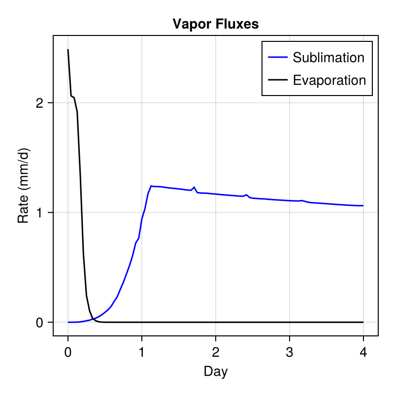

fig2 = Figure(size = (800, 1200))
ax1 = Axis(fig2[1, 1], title = "Temperature")
CairoMakie.ylims!(-0.35, 0)
CairoMakie.xlims!(260, 280)
linestyles = [:solid, :dash, :dashdot, :dashdotdot, :dot]
days = [0, 1, 2, 3, 4]
for i in 1:length(days)
    CairoMakie.lines!(
        ax1,
        parent(sv.saveval[Int(days[i] * 24 + 1)].soil.T)[:],
        parent(z)[:],
        label = "$(days[i]) days",
        color = :black,
        linestyle = linestyles[i],
    )
end
ax2 = Axis(fig2[2, 1], title = "Ice", ylabel = "Depth(cm)")

CairoMakie.ylims!(-0.35, 0)
CairoMakie.xlims!(0.0, 0.5)
for i in 1:length(days)
    CairoMakie.lines!(
        ax2,
        parent(sol.u[Int(days[i] * 24 + 1)].soil.θ_i)[:],
        parent(z)[:],
        label = "$(days[i]) days",
        color = :black,
        linestyle = linestyles[i],
    )
end
ax3 = Axis(fig2[3, 1], title = "Liquid Water", xlabel = "")
CairoMakie.ylims!(-0.35, 0)
CairoMakie.xlims!(0.0, 0.5)
for i in 1:length(days)
    CairoMakie.lines!(
        ax3,
        parent(sol.u[Int(days[i] * 24 + 1)].soil.ϑ_l)[:],
        parent(z)[:],
        label = "$(days[i]) days",
        color = :black,
        linestyle = linestyles[i],
    )
end

CairoMakie.axislegend(ax3, position = :lt)
CairoMakie.axislegend(ax2, position = :lt)
CairoMakie.axislegend(ax1, position = :lt)
save("profiles.png", fig2);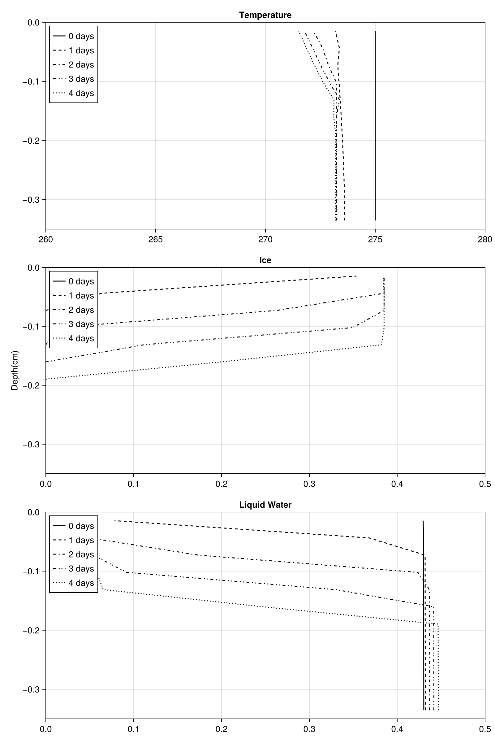

This page was generated using Literate.jl.