Convergence Tests

Convergence tests are implemented in /validation/convergence_tests and range from zero-dimensional time-stepper tests to two-dimensional integration tests that involve non-trivial pressure fields, advection, and diffusion.

For all tests except point exponential decay, we use the norm,

and norm,

to compare simulated fields, , with exact, analytically-derived solutions . The field may be a tracer field or a velocity field.

Point Exponential Decay

This test analyzes time-stepper convergence by simulating the zero-dimensional, or spatially-uniform equation

with the initial condition  , which has the analytical solution  .

We find the expected first-order convergence with decreasing time-step using our first-order accurate, "modified second-order" Adams-Bashforth time-stepping method:

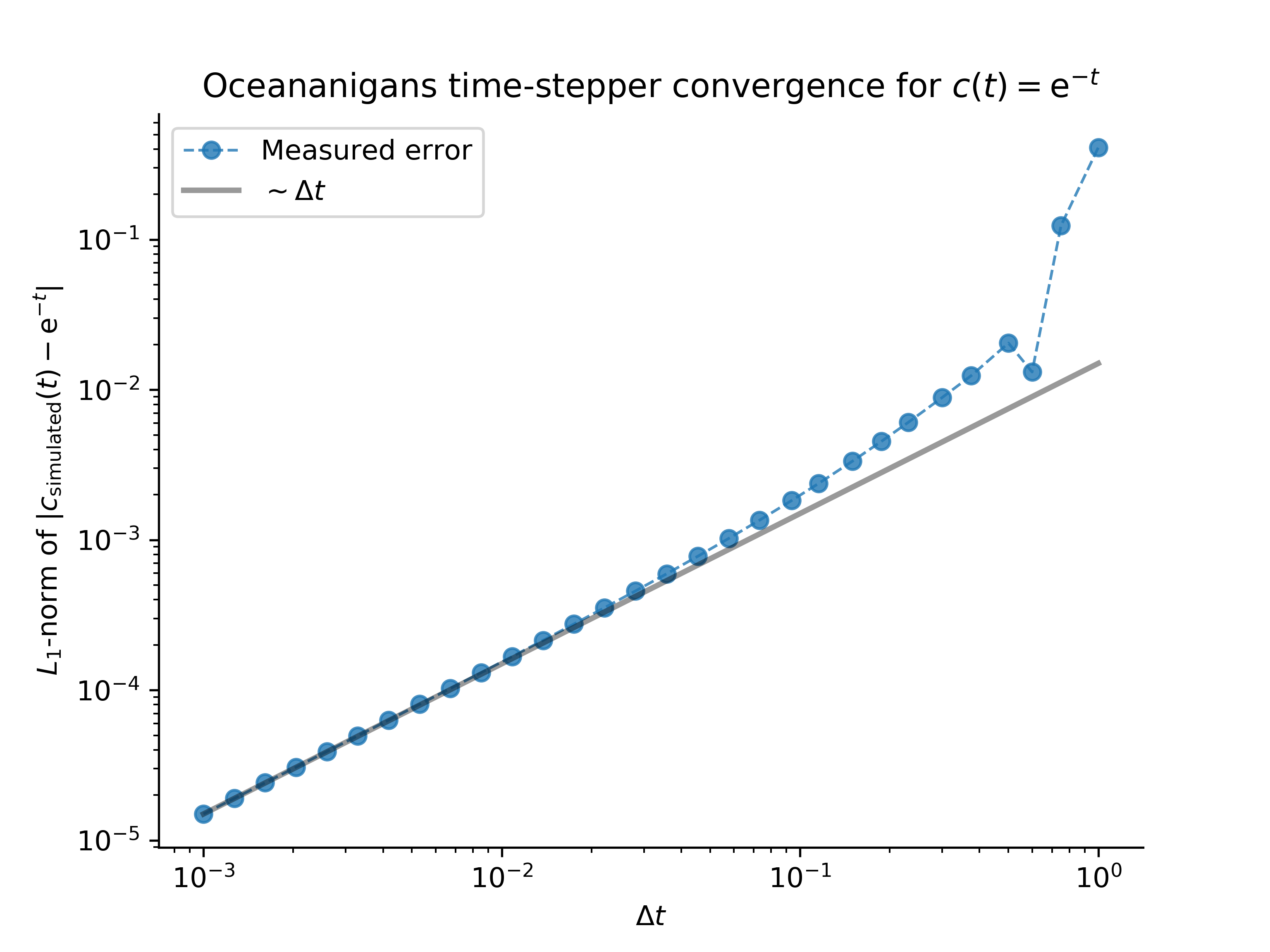
This result validates the correctness of the Oceananigans implementation of Adams-Bashforth time-stepping.

One-dimensional advection and diffusion of a Gaussian

This and the following tests focus on convergence with grid spacing, .

In one dimension with constant diffusivity and in the presence of a constant velocity , a Gaussian evolves according to

For this test we take the initial time as  . We simulate this problem with advection and diffusion, as well as with   and thus diffusion only, as well as with   and thus "advection only". The solutions are

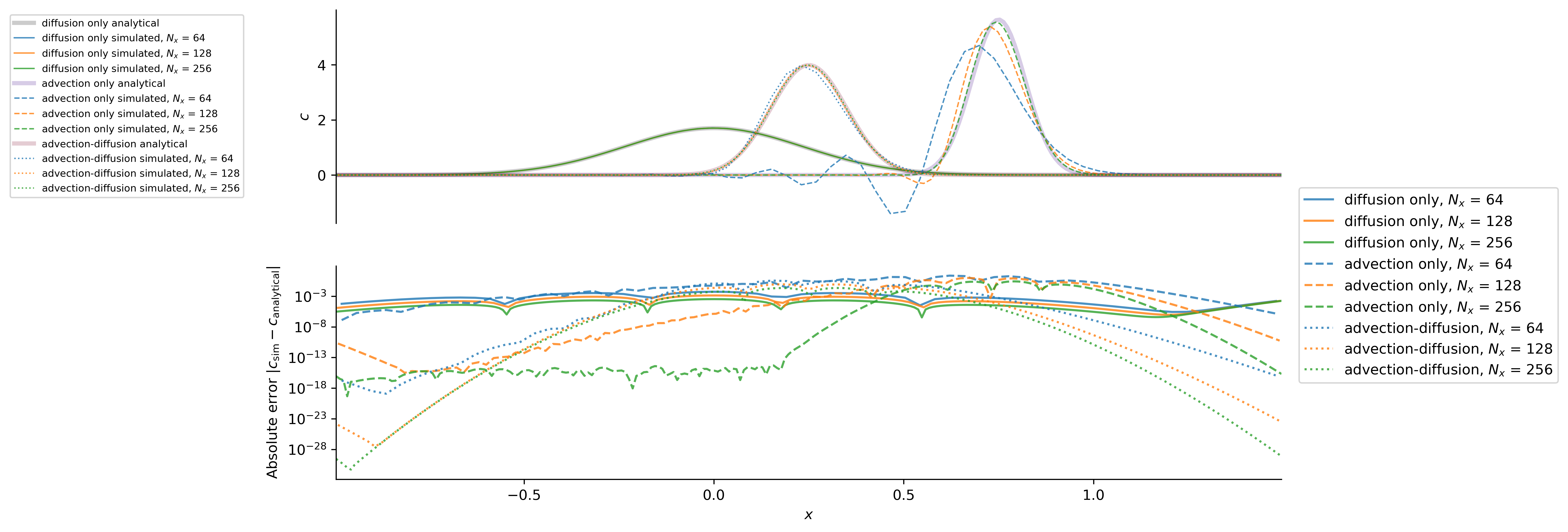
which exhibit the expected second-order convergence with  :

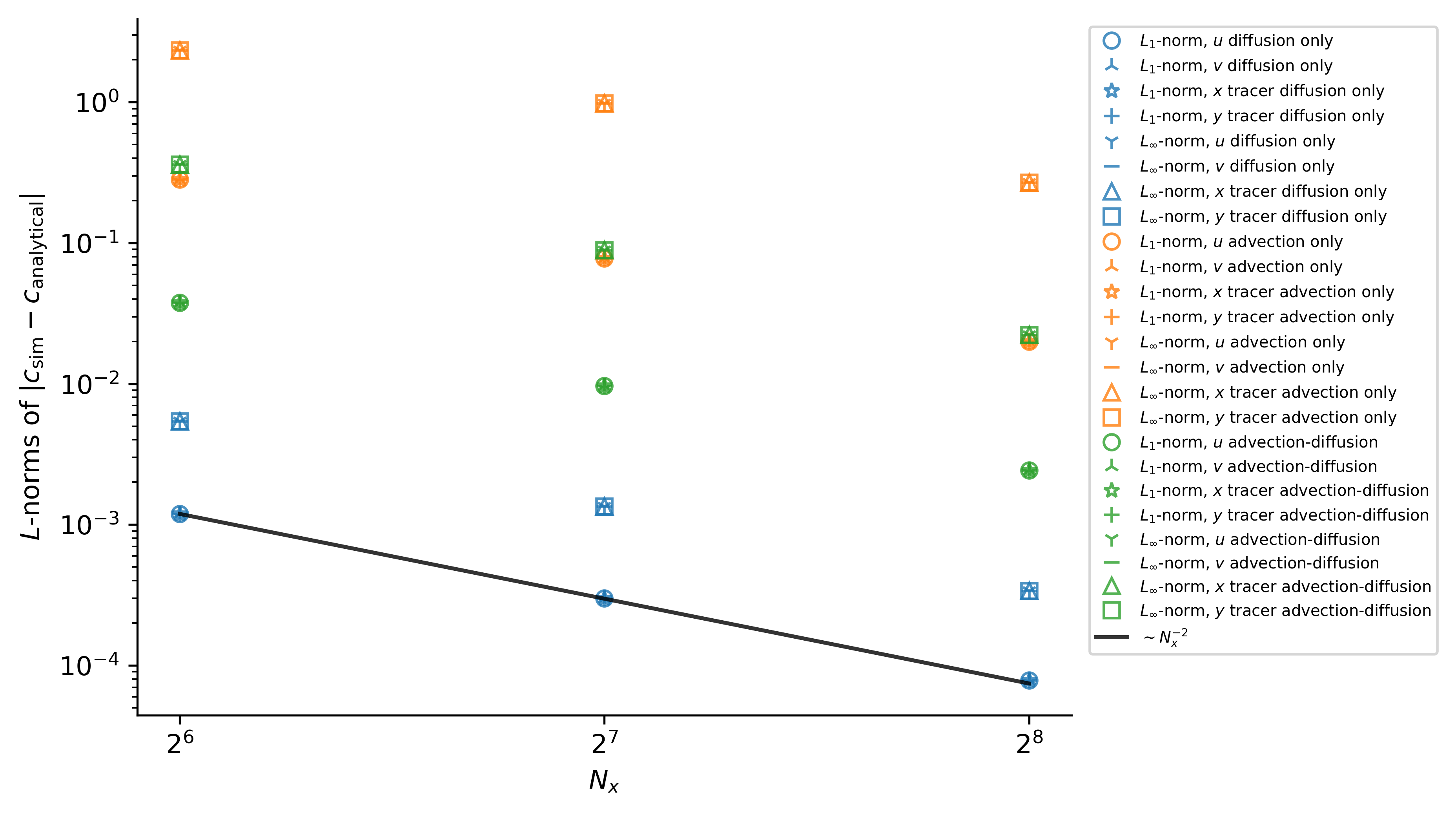
These results validate the correctness of time-stepping, constant diffusivity operators, and advection operators.

One-dimensional advection and diffusion of a cosine

In one dimension with constant diffusivity and in the presence of a constant velocity , a cosine evolves according to

The solutions are

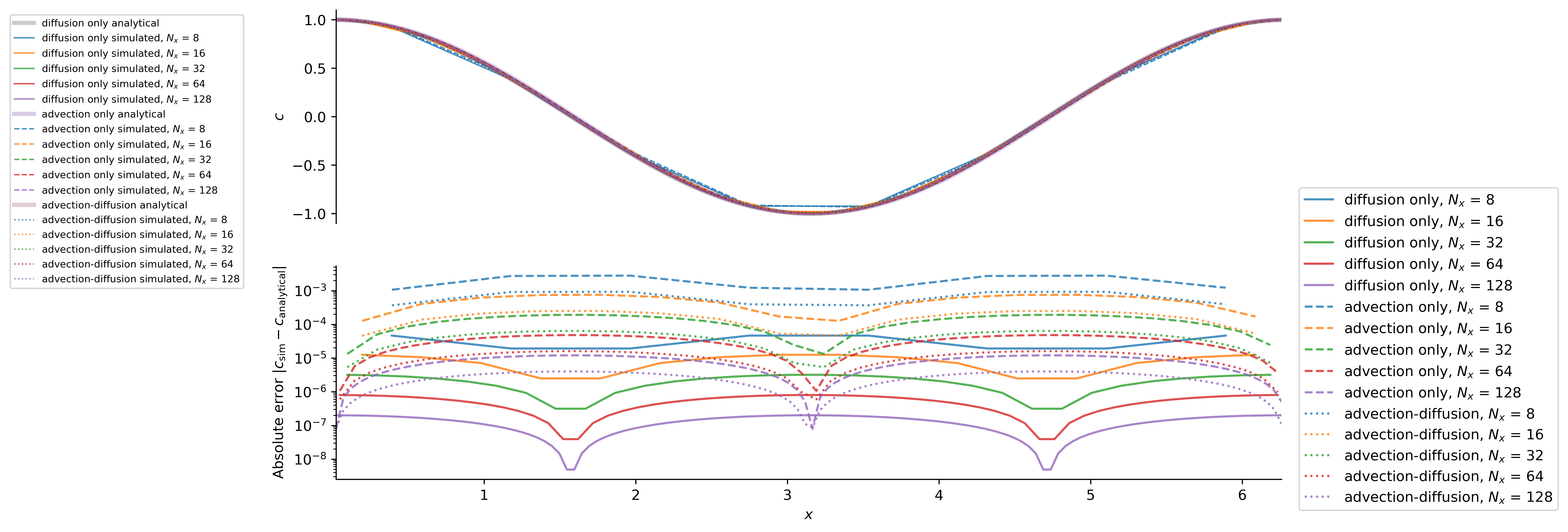
which exhibit the expected second-order convergence with  :

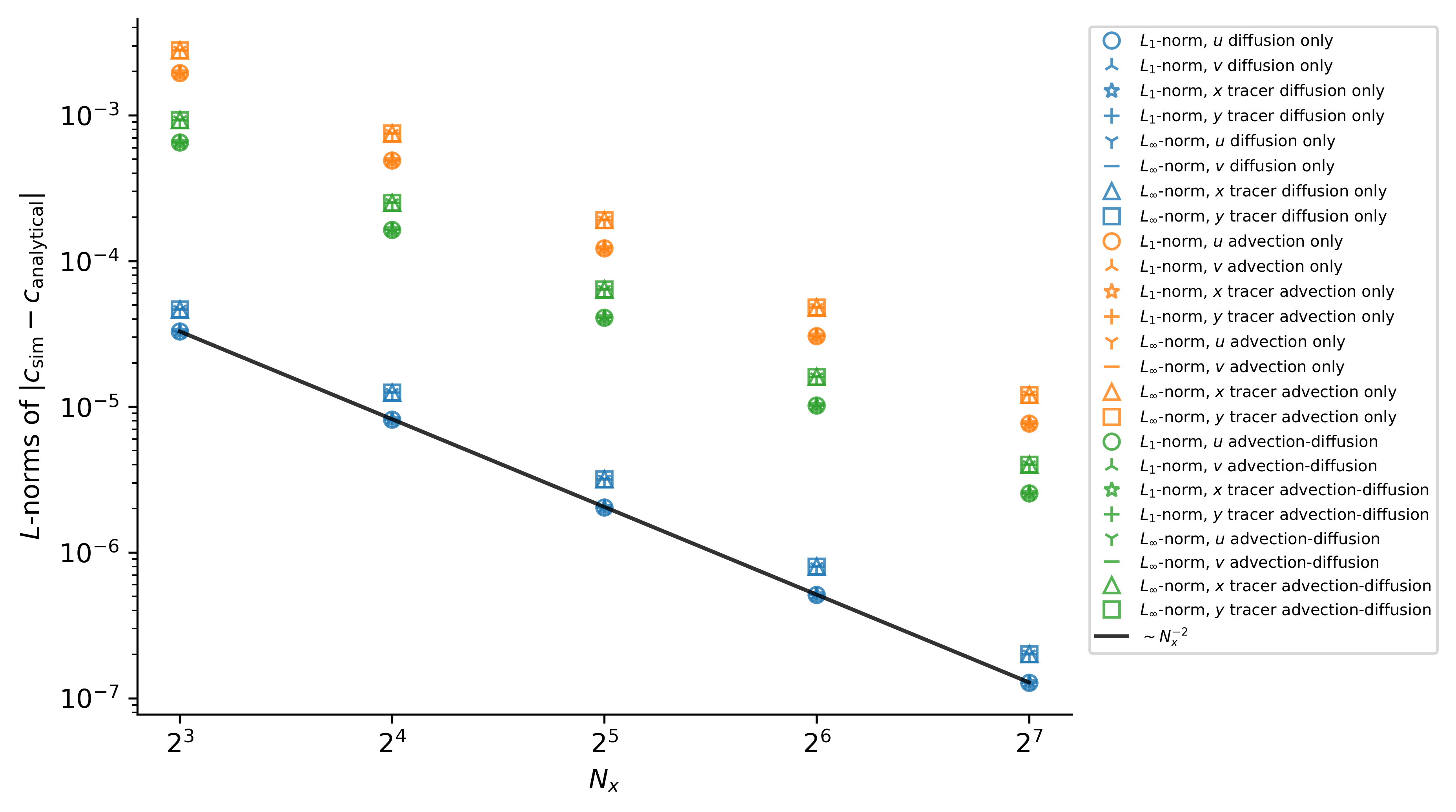
These results validate the correctness of time-stepping, constant diffusivity operators, and advection operators.

Two-dimensional diffusion

With zero velocity field and constant diffusivity , the tracer field

decays according to

with either periodic boundary conditions, or insulating boundary conditions in either or .

The expected convergence with   is observed:

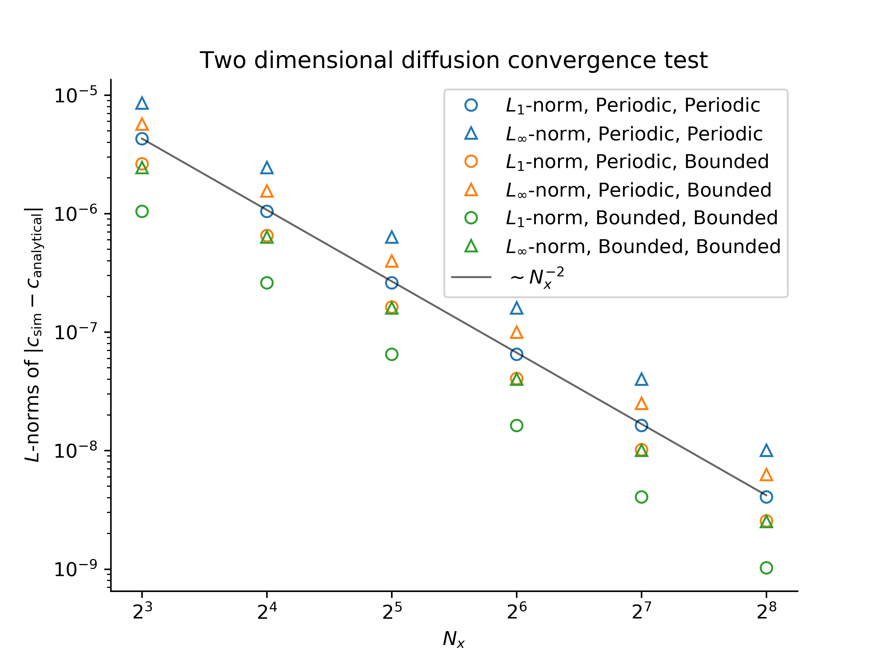
This validates the correctness of multi-dimensional diffusion operators.

Decaying, advected Taylor-Green vortex

The velocity field

is a solution to the Navier-Stokes equations with viscosity  .

The expected convergence with spatial resolution is observed:

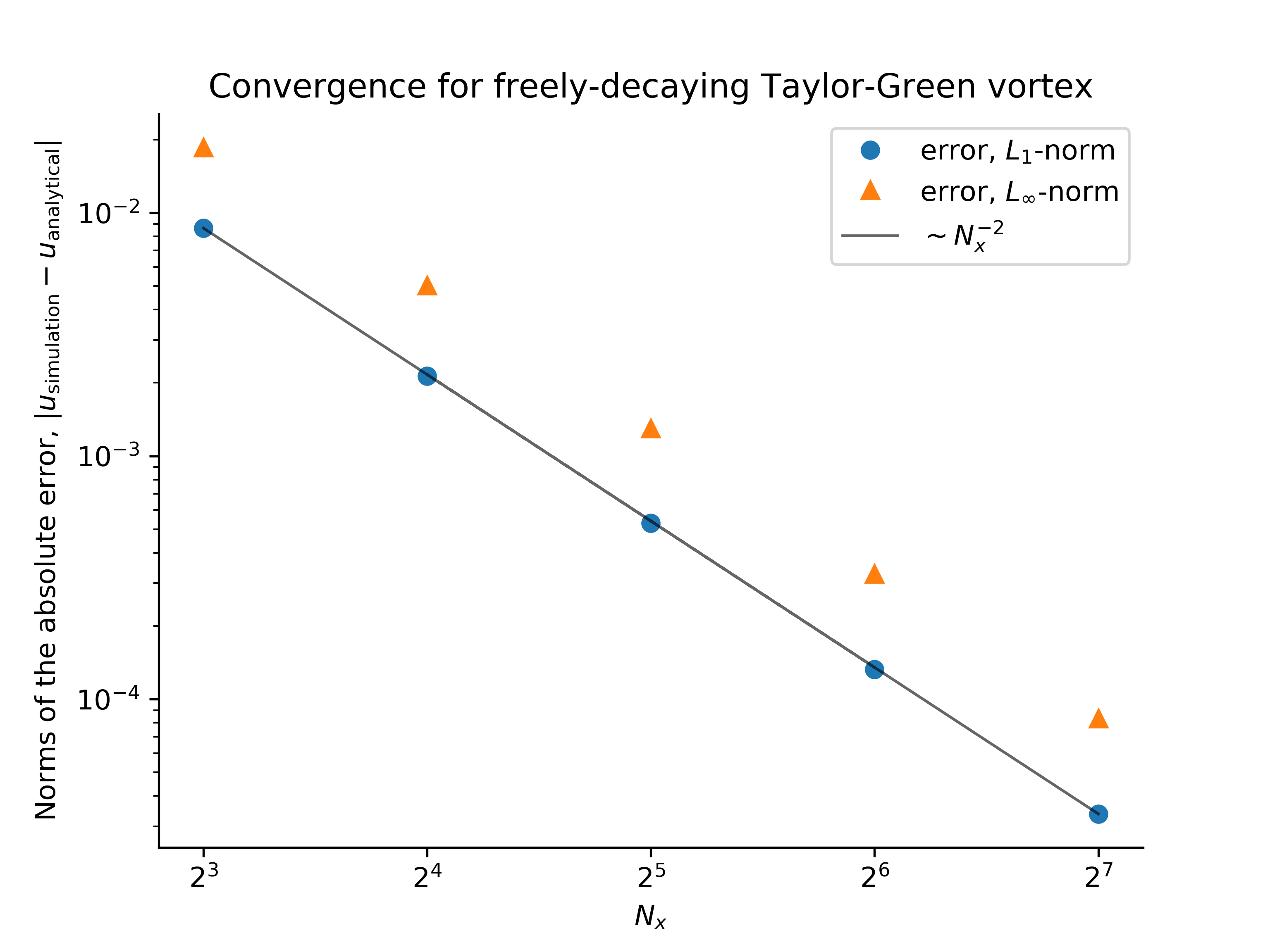
This validates the correctness of the advection and diffusion of a velocity field.

Forced two-dimensional flows

We introduce two convergence tests associated with forced flows in domains that are bounded in , and periodic in with no tracers.

Note: in this section, subscripts are used to denote derivatives to make reading and typing equations easier.

In a two-dimensional flow in , the velocity field can be expressed in terms of a streamfunction such that

where subscript denote derivatives such that  , for example. With an isotropic Laplacian viscosity  , the momentum and continuity equations are

while the equation for vorticity,    , is

Finally, taking the divergence of the momentum equation, we find a Poisson equation for pressure,

To pose the problem, we first pick a streamfunction . This choice then yields the vorticity forcing that satisfies the vorticity equation. We then determine by solving   , and pick so that we can solve the Poisson equation for pressure.

We restrict ourselves to a class of problems in which

Grinding through the algebra, this particular form implies that is given by

where primes denote derivatives of functions of a single argument. Setting  , we find that if satisfies

then the pressure Poisson equation becomes

This completes the specification of the problem.

We set up the problem by imposing the time-dependent forcing functions and on and , initializing the flow at  , and integrating the problem forwards in time using Oceananigans. We find the expected convergence of the numerical solution to the analytical solution: the error between the numerical and analytical solutions decreases with  , where is the number of grid points and is the spatial resolution:

The convergence tests are performed using both and as the bounded direction.

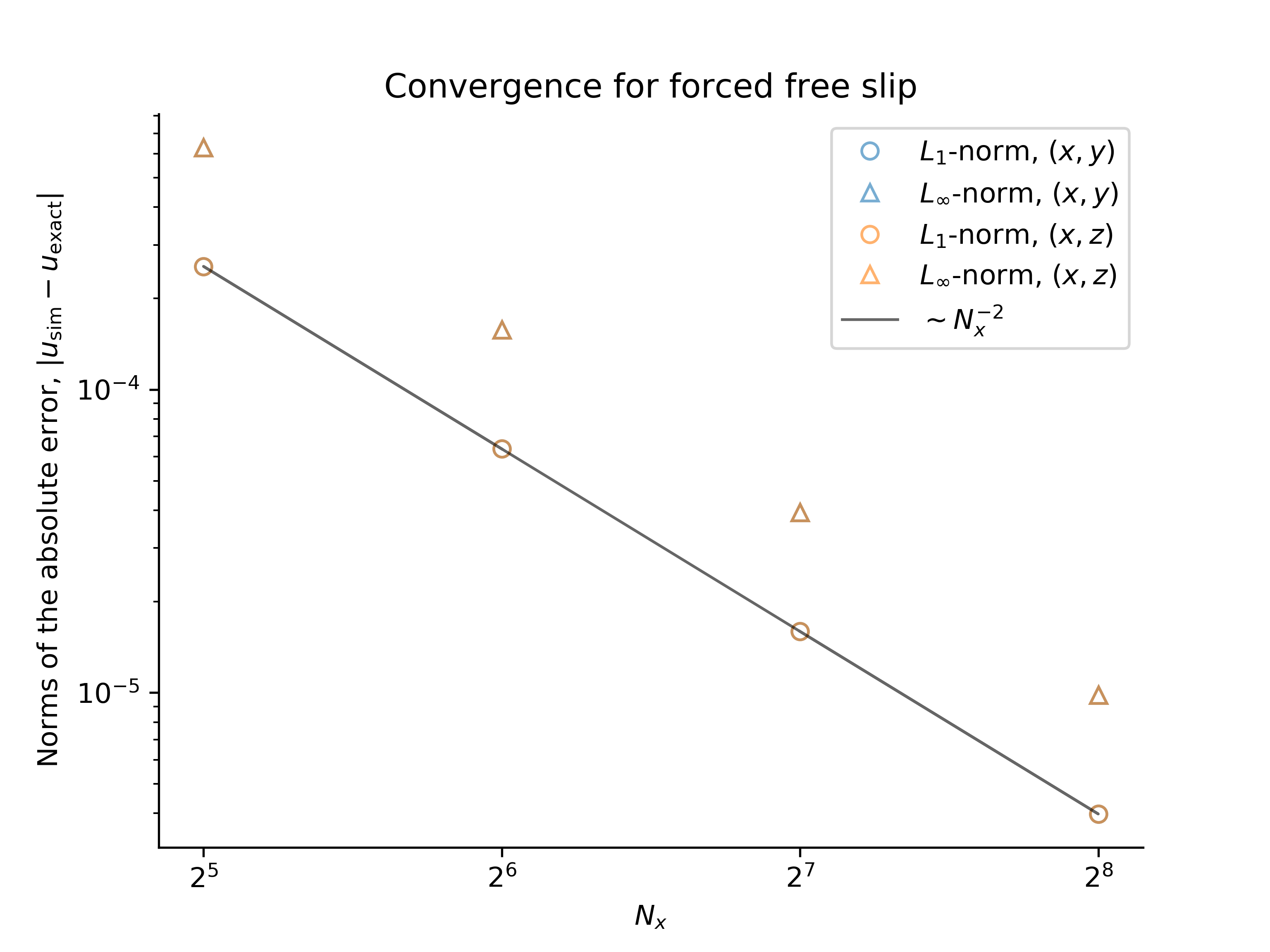
Forced, free-slip flow

A forced flow satisfying free-slip conditions at   and   has the streamfunction

and thus  . The velocity field is

which satisfies the boundary conditions    and   . The vorticity forcing is

which implies that

and  .

Forced, fixed-slip flow

A forced flow satisfying "fixed-slip" boundary conditions at   and   has the streamfunction

and thus   . The velocity field is

which satisfies the boundary conditions

The vorticity forcing is

which implies that

and

We set up the problem in the same manner as the forced, free-slip problem above. Note that we also must the no-slip boundary condition   and the time-dependent fixed-slip condition  . As for the free-slip problem, we find that the error between the numerical and analytical solutions decreases with  , where is the number of grid points and is the spatial resolution:

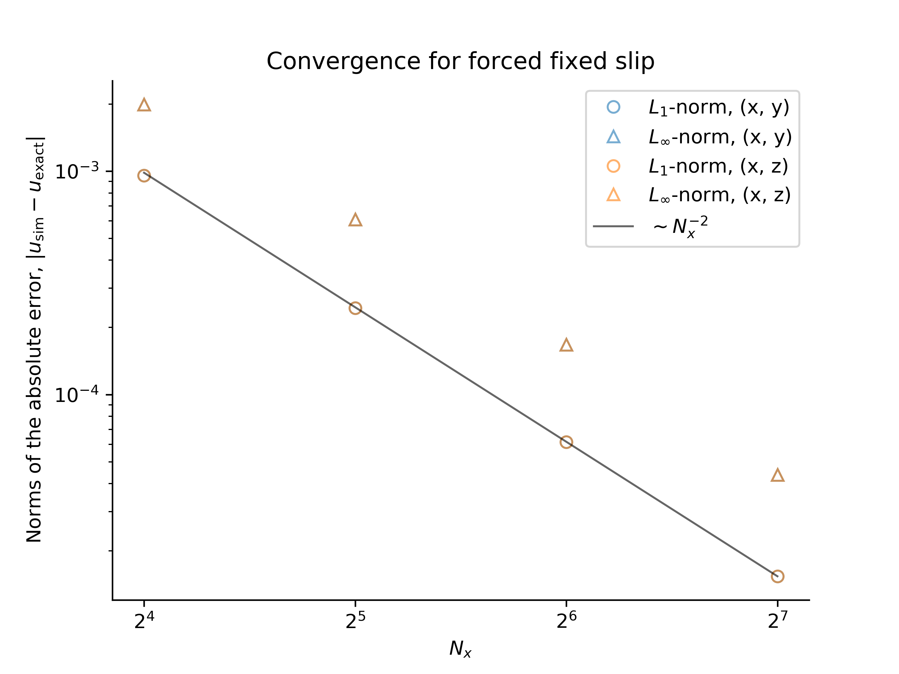
The convergence tests are performed using both and as the bounded direction.