Fields basics

Fields and its relatives are core Oceananigans data structures. Fields are arrays of data located on a grid, whose entries correspond to the average value of some quantity over some finite-sized volume. Fields also may contain boundary_conditions, may be computed from an operand or expression involving other fields, and may cover only a portion of the total indices spanned by the grid.

Staggered grids and field locations

Oceananigans ocean-flavored fluids simulations rely fundamentally on "staggered grid" numerical methods.

Recall that grids represent a physical domain divided into finite volumes. For example, let's consider a horizontally-periodic, vertically-bounded grid of cells that divide up a cube with dimensions   :

using Oceananigans

grid = RectilinearGrid(topology = (Periodic, Periodic, Bounded),
                       size = (4, 5, 4),
                       halo = (1, 1, 1),
                       x = (0, 1),
                       y = (0, 1),
                       z = [0, 0.1, 0.3, 0.6, 1])

# output
4×5×4 RectilinearGrid{Float64, Periodic, Periodic, Bounded} on CPU with 1×1×1 halo
├── Periodic x ∈ [0.0, 1.0) regularly spaced with Δx=0.25
├── Periodic y ∈ [0.0, 1.0) regularly spaced with Δy=0.2
└── Bounded  z ∈ [0.0, 1.0] variably spaced with min(Δz)=0.1, max(Δz)=0.4

The cubic domain is divided into a "primary mesh" of     cells, which are evenly spaced in but variably spaced in . Now, in addition to the primary mesh, the grid defines also a set of "staggered" grids whose cells are shifted by half a cell width relative to the primary mesh. In other words, the staggered grid cells have a "location" in each direction – either Center, and therefore co-located with the primary mesh, or Face and located over the interfaces of the primary mesh. For example, the primary or Center cell spacings in are

zspacings(grid, Center())[:, :, 1:4]

# output
4-element Vector{Float64}:
 0.1
 0.19999999999999998
 0.3
 0.4

corresponding to cell interfaces located at z = [0, 0.1, 0.3, 0.6, 1]. But then for the grid which is staggered in z relative to the primary mesh,

zspacings(grid, Face())[:, :, 1:5]

# output
5-element Vector{Float64}:
 0.1
 0.15000000000000002
 0.24999999999999994
 0.3500000000000001
 0.3999999999999999

The cells for the vertically staggered grid have different spacings than the primary mesh. That's because the edges of the vertically-staggered mesh coincide with the nodes (the cell centers) of the primary mesh. The nodes of the primary mesh are

znodes(grid, Center(), with_halos=true)

# output
6-element view(OffsetArray(::Vector{Float64}, 0:5), :) with eltype Float64 with indices 0:5:
 -0.05
  0.05
  0.2
  0.44999999999999996
  0.8
  1.2

The center of the leftmost "halo cell" is z = -0.05, while the center of the first cell from the left is z = 0.05. This means that the width of the first cell on the vertically-staggered grid is 0.05 - (-0.05) = 0.1 – and so on. Finally, note that the nodes of the staggered mesh coincide with the cell interfaces of the primary mesh, so:

znodes(grid, Center())

# output
4-element view(::Vector{Float64}, 2:5) with eltype Float64:
 0.05
 0.2
 0.44999999999999996
 0.8

In a three-dimensional domain, there are    meshes – 1 primary mesh, and 7 meshes that are staggered to varying degrees from the primary mesh. This system of staggered grids is commonly used in fluid dynamics and was invented specifically for simulations of the atmosphere and ocean.

Constructing Fields at specified locations

Every Field is associated with either the primary mesh or one of the staggered meshes by a three-dimensional "location" associated with each field. To build a fully-centered Field, for example, we write

c = Field{Center, Center, Center}(grid)

# output
4×5×4 Field{Center, Center, Center} on RectilinearGrid on CPU
├── grid: 4×5×4 RectilinearGrid{Float64, Periodic, Periodic, Bounded} on CPU with 1×1×1 halo
├── boundary conditions: FieldBoundaryConditions
│   └── west: Periodic, east: Periodic, south: Periodic, north: Periodic, bottom: ZeroFlux, top: ZeroFlux, immersed: Nothing
└── data: 6×7×6 OffsetArray(::Array{Float64, 3}, 0:5, 0:6, 0:5) with eltype Float64 with indices 0:5×0:6×0:5
    └── max=0.0, min=0.0, mean=0.0

Fully-centered fields also go by the alias CenterField,

c == CenterField(grid)

# output
true

Many fluid dynamical variables are located at cell centers – for example, tracers like temperature and salinity. Another common type of Field we encounter have cells located over the x-interfaces of the primary grid,

u = Field{Face, Center, Center}(grid)

# output
4×5×4 Field{Face, Center, Center} on RectilinearGrid on CPU
├── grid: 4×5×4 RectilinearGrid{Float64, Periodic, Periodic, Bounded} on CPU with 1×1×1 halo
├── boundary conditions: FieldBoundaryConditions
│   └── west: Periodic, east: Periodic, south: Periodic, north: Periodic, bottom: ZeroFlux, top: ZeroFlux, immersed: Nothing
└── data: 6×7×6 OffsetArray(::Array{Float64, 3}, 0:5, 0:6, 0:5) with eltype Float64 with indices 0:5×0:6×0:5
    └── max=0.0, min=0.0, mean=0.0

which also goes by the alias u = XFaceField(grid). The name u is suggestive: in the Arakawa type-C grid ('C-grid' for short) used by Oceananigans, the x-component of the velocity field is stored at Face, Center, Center location.

The centers of the u cells are shifted to the left relative to the c cells:

@show collect(xnodes(c))
@show collect(xnodes(u))
nothing

# output
collect(xnodes(c)) = [0.125, 0.375, 0.625, 0.875]
collect(xnodes(u)) = [0.0, 0.25, 0.5, 0.75]

Notice that the first u-node is at x=0, the left end of the grid, but the last u-node is at x=0.75. Because the x-direction is Periodic, the XFaceField u has 4 cells in x – the cell just right of x=0.75 is the same as the cell at x=0.

Because the vertical direction is Bounded, however, vertically-staggered fields have more vertical cells than CenterFields:

w = Field{Center, Center, Face}(grid)

@show collect(znodes(c))
@show collect(znodes(w))
nothing

# output
collect(znodes(c)) = [0.05, 0.2, 0.44999999999999996, 0.8]
collect(znodes(w)) = [0.0, 0.1, 0.3, 0.6, 1.0]

Fields at Center, Center, Face are also called ZFaceField, and the vertical velocity is a ZFaceField on the C-grid. Let's visualize the situation:

using CairoMakie

fig = Figure(size=(600, 180))
ax = Axis(fig[1, 1], xlabel="x")

# Visualize the domain
lines!(ax, [0, 1], [0, 0], color=:gray)

xc = xnodes(c)
xu = xnodes(u)

scatter!(ax, xc, 0 * xc, marker=:circle, markersize=10, label="Cell centers")
scatter!(ax, xu, 0 * xu, marker=:vline, markersize=20, label="Cell interfaces")

ylims!(ax, -1, 1)
xlims!(ax, -0.1, 1.1)
hideydecorations!(ax)
hidexdecorations!(ax, ticklabels=false, label=false)
hidespines!(ax)

Legend(fig[0, 1], ax, nbanks=2, framevisible=false)

current_figure()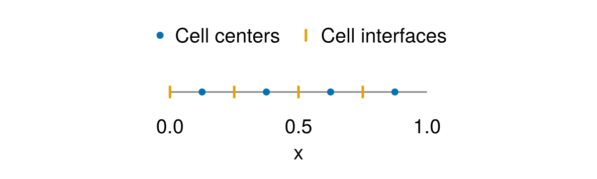

Setting Fields

Fields are full of 0's when they are created, which is not very exciting. The situation can be improved using set! to change the values of a field. For example,

set!(c, 42)

# output
4×5×4 Field{Center, Center, Center} on RectilinearGrid on CPU
├── grid: 4×5×4 RectilinearGrid{Float64, Periodic, Periodic, Bounded} on CPU with 1×1×1 halo
├── boundary conditions: FieldBoundaryConditions
│   └── west: Periodic, east: Periodic, south: Periodic, north: Periodic, bottom: ZeroFlux, top: ZeroFlux, immersed: Nothing
└── data: 6×7×6 OffsetArray(::Array{Float64, 3}, 0:5, 0:6, 0:5) with eltype Float64 with indices 0:5×0:6×0:5
    └── max=42.0, min=42.0, mean=42.0

Now c is filled with 42s (for this simple case, we could also have used c .= 42). Let's confirm that:

c[1, 1, 1]

# output
42.0

Looks good. And

c[1:4, 1:5, 1]

# output
4×5 Matrix{Float64}:
 42.0  42.0  42.0  42.0  42.0
 42.0  42.0  42.0  42.0  42.0
 42.0  42.0  42.0  42.0  42.0
 42.0  42.0  42.0  42.0  42.0

Note that indexing into c is the same as indexing into c.data.

c[:, :, :] == c.data

# output
true

We can also set! with arrays,

random_stuff = rand(size(c)...)
set!(c, random_stuff)

heatmap(view(c, :, :, 1))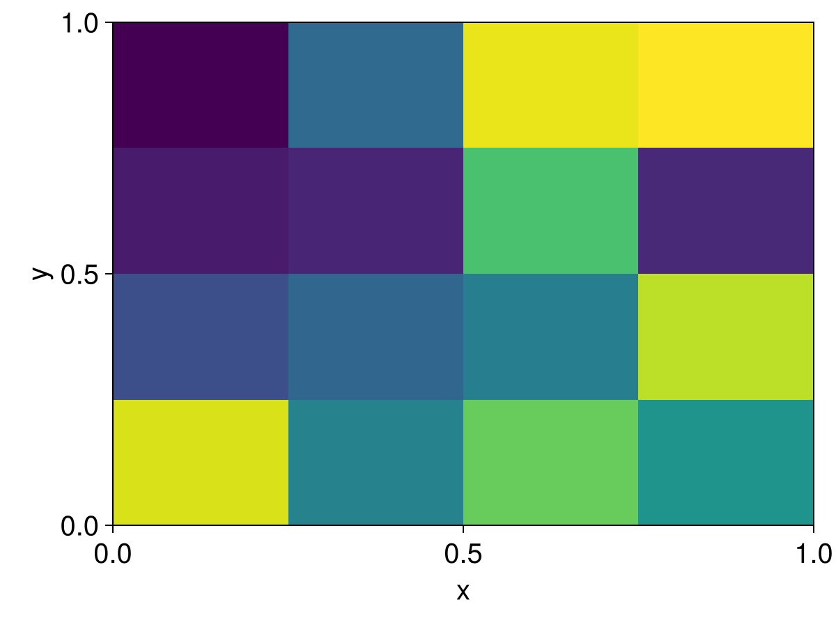

or even use functions to set,

fun_stuff(x, y, z) = 2x
set!(c, fun_stuff)

# output
4×5×4 Field{Center, Center, Center} on RectilinearGrid on CPU
├── grid: 4×5×4 RectilinearGrid{Float64, Periodic, Periodic, Bounded} on CPU with 1×1×1 halo
├── boundary conditions: FieldBoundaryConditions
│   └── west: Periodic, east: Periodic, south: Periodic, north: Periodic, bottom: ZeroFlux, top: ZeroFlux, immersed: Nothing
└── data: 6×7×6 OffsetArray(::Array{Float64, 3}, 0:5, 0:6, 0:5) with eltype Float64 with indices 0:5×0:6×0:5
    └── max=1.75, min=0.25, mean=1.0

and plot it

heatmap(view(c, :, :, 1))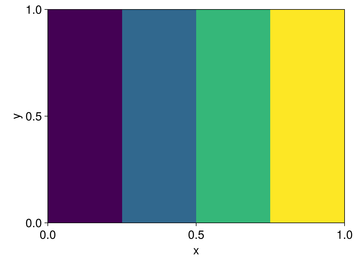

For Fields on three-dimensional grids, set! functions must have arguments x, y, z for RectilinearGrid, or λ, φ, z for LatitudeLongitudeGrid and OrthogonalSphericalShellGrid. But for Fields on one- and two-dimensional grids, only the arguments that correspond to the non-Flat directions must be included. For example, to set! on a one-dimensional grid we write

# Make a field on a one-dimensional grid
one_d_grid = RectilinearGrid(size=7, x=(0, 7), topology=(Periodic, Flat, Flat))
one_d_c = CenterField(one_d_grid)

# The one-dimensional grid varies only in `x`
still_pretty_fun(x) = 3x
set!(one_d_c, still_pretty_fun)

# output
7×1×1 Field{Center, Center, Center} on RectilinearGrid on CPU
├── grid: 7×1×1 RectilinearGrid{Float64, Periodic, Flat, Flat} on CPU with 3×0×0 halo
├── boundary conditions: FieldBoundaryConditions
│   └── west: Periodic, east: Periodic, south: Nothing, north: Nothing, bottom: Nothing, top: Nothing, immersed: Nothing
└── data: 13×1×1 OffsetArray(::Array{Float64, 3}, -2:10, 1:1, 1:1) with eltype Float64 with indices -2:10×1:1×1:1
    └── max=19.5, min=1.5, mean=10.5

Note

Field data is always stored in three-dimensional arrays –- even when they have Nothing locations, or on grids with Flat directions. As a result, Fields are indexed with three indices i, j, k, with Flat directions indexed with 1.

A bit more about setting with functions

Let's return to the three-dimensional fun_stuff case to investigate in more detail how set! works with functions. The xnodes of c – the coordinates of the center of c's finite volumes – are:

xc = xnodes(c)
@show collect(xc)
nothing # hide

# output
collect(xc) = [0.125, 0.375, 0.625, 0.875]

To set! the values of c we evaluate fun_stuff at c's nodes, producing

c[1:4, 1, 1]

# output
4-element Vector{Float64}:
 0.25
 0.75
 1.25
 1.75

Note

This function-setting method is a first-order method for computing the finite volume of c to fun_stuff. Higher-order algorithms could be implemented – have a crack if you're keen.

As a result set! can evaluate differently on Fields at different locations:

u = XFaceField(grid)
set!(u, fun_stuff)
u[1:4, 1, 1]

# output
4-element Vector{Float64}:
 0.0
 0.5
 1.0
 1.5

Halo regions and boundary conditions

We built grid with halo = (1, 1, 1), which means that the "interior" cells of the grid are surrounded by a "halo region" of cells that's one cell thick. The number of halo cells in each direction are stored in the properties Hx, Hy, Hz, so,

(grid.Hx, grid.Hy, grid.Hz)

# output
(1, 1, 1)

set! doesn't touch halo cells. Check out one of the two-dimensional slices of c showing both the interior and the halo regions:

c[:, :, 1]

# output
6×7 OffsetArray(::Matrix{Float64}, 0:5, 0:6) with eltype Float64 with indices 0:5×0:6:
 0.0  0.0   0.0   0.0   0.0   0.0   0.0
 0.0  0.25  0.25  0.25  0.25  0.25  0.0
 0.0  0.75  0.75  0.75  0.75  0.75  0.0
 0.0  1.25  1.25  1.25  1.25  1.25  0.0
 0.0  1.75  1.75  1.75  1.75  1.75  0.0
 0.0  0.0   0.0   0.0   0.0   0.0   0.0

The interior region is populated, but the surrounding halo regions are all 0. To remedy this situation we need to fill_halo_regions!:

using Oceananigans.BoundaryConditions: fill_halo_regions!

fill_halo_regions!(c)

c[:, :, 1]

# output
6×7 OffsetArray(::Matrix{Float64}, 0:5, 0:6) with eltype Float64 with indices 0:5×0:6:
 1.75  1.75  1.75  1.75  1.75  1.75  1.75
 0.25  0.25  0.25  0.25  0.25  0.25  0.25
 0.75  0.75  0.75  0.75  0.75  0.75  0.75
 1.25  1.25  1.25  1.25  1.25  1.25  1.25
 1.75  1.75  1.75  1.75  1.75  1.75  1.75
 0.25  0.25  0.25  0.25  0.25  0.25  0.25

The way the halo regions are filled depends on c.boundary_conditions:

c.boundary_conditions

# output
Oceananigans.FieldBoundaryConditions, with boundary conditions
├── west: PeriodicBoundaryCondition
├── east: PeriodicBoundaryCondition
├── south: PeriodicBoundaryCondition
├── north: PeriodicBoundaryCondition
├── bottom: FluxBoundaryCondition: Nothing
├── top: FluxBoundaryCondition: Nothing
└── immersed: Nothing

Specifically for c above, x and y are Periodic while z has been assigned the default "no-flux" boundary conditions for a Field with Center location in a Bounded direction. For no-flux boundary conditions, the halo regions of c are filled so that derivatives evaluated on the boundary return 0. To view only the interior cells of c we use the function interior,

interior(c, :, :, 1)

# output
4×5 view(::Array{Float64, 3}, 2:5, 2:6, 2) with eltype Float64:
 0.25  0.25  0.25  0.25  0.25
 0.75  0.75  0.75  0.75  0.75
 1.25  1.25  1.25  1.25  1.25
 1.75  1.75  1.75  1.75  1.75

Note that the indices of c (and the indices of c.data) are "offset" so that index 1 corresponds to the first interior cell. As a result,

c[1:4, 1:5, 1] == interior(c, :, :, 1)

# output
true

and more generally

typeof(c.data)

# output
OffsetArrays.OffsetArray{Float64, 3, Array{Float64, 3}}

Thus, for example, the x-indices of c.data vary from 1 - Hx to Nx + Hx – in this case, from 0 to 5. The underlying array can be accessed with parent(c). But note that the "parent" array does not have offset indices, so

@show parent(c)[1:2, 2, 2]
@show c.data[1:2, 1, 1]
nothing

# output
(parent(c))[1:2, 2, 2] = [1.75, 0.25]
c.data[1:2, 1, 1] = [0.25, 0.75]

Reduced-dimension fields with indices

By default, Fields span the full extent of the grid: their indices are (:, :, :). But sometimes we want a field that lives on only a slice of the grid – for example, a two-dimensional horizontal field representing the surface vorticity, or a one-dimensional field along a single column. This is achieved by passing the indices keyword argument to the Field constructor.

For example, to create a two-dimensional - field at the top of the domain (corresponding to the last Center index, k = grid.Nz):

surface_c = Field{Center, Center, Center}(grid, indices=(:, :, grid.Nz))

# output
4×5×1 Field{Center, Center, Center} on RectilinearGrid on CPU
├── grid: 4×5×4 RectilinearGrid{Float64, Periodic, Periodic, Bounded} on CPU with 1×1×1 halo
├── boundary conditions: FieldBoundaryConditions
│   └── west: Periodic, east: Periodic, south: Periodic, north: Periodic, bottom: Nothing, top: Nothing, immersed: Nothing
├── indices: (:, :, 4:4)
└── data: 6×7×1 OffsetArray(::Array{Float64, 3}, 0:5, 0:6, 4:4) with eltype Float64 with indices 0:5×0:6×4:4
    └── max=0.0, min=0.0, mean=0.0

Notice that the resulting field is 4×5×1 instead of 4×5×4 – it occupies only a single index in the vertical. Also notice the indices: (:, :, 4:4) line in the output: the integer index grid.Nz = 4 has been converted to the range 4:4.

We can set! reduced fields the same way as full fields:

set!(surface_c, (x, y, z) -> x + y)

surface_c[1:4, 1:5, grid.Nz]

# output
4×5 Matrix{Float64}:
 0.225  0.425  0.625  0.825  1.025
 0.475  0.675  0.875  1.075  1.275
 0.725  0.925  1.125  1.325  1.525
 0.975  1.175  1.375  1.575  1.775

Reduced fields from operations

The indices keyword is particularly useful in combination with field operations. For example, suppose we want to compute and store the vertical vorticity   only at the surface:

u = XFaceField(grid)
v = YFaceField(grid)

ωₛ = Field(∂x(v) - ∂y(u), indices=(:, :, grid.Nz))

# output
4×5×1 Field{Face, Face, Center} on RectilinearGrid on CPU
├── grid: 4×5×4 RectilinearGrid{Float64, Periodic, Periodic, Bounded} on CPU with 1×1×1 halo
├── boundary conditions: FieldBoundaryConditions
│   └── west: Periodic, east: Periodic, south: Periodic, north: Periodic, bottom: Nothing, top: Nothing, immersed: Nothing
├── indices: (:, :, 4:4)
├── operand: BinaryOperation at (Face, Face, Center)
├── status: time=0.0
└── data: 6×7×1 OffsetArray(::Array{Float64, 3}, 0:5, 0:6, 4:4) with eltype Float64 with indices 0:5×0:6×4:4
    └── max=0.0, min=0.0, mean=0.0

Computing ωₛ with compute! evaluates the expression ∂x(v) - ∂y(u) and stores the result only at the surface slice:

compute!(ωₛ)

# output
4×5×1 Field{Face, Face, Center} on RectilinearGrid on CPU
├── grid: 4×5×4 RectilinearGrid{Float64, Periodic, Periodic, Bounded} on CPU with 1×1×1 halo
├── boundary conditions: FieldBoundaryConditions
│   └── west: Periodic, east: Periodic, south: Periodic, north: Periodic, bottom: Nothing, top: Nothing, immersed: Nothing
├── indices: (:, :, 4:4)
├── operand: BinaryOperation at (Face, Face, Center)
├── status: time=0.0
└── data: 6×7×1 OffsetArray(::Array{Float64, 3}, 0:5, 0:6, 4:4) with eltype Float64 with indices 0:5×0:6×4:4
    └── max=0.0, min=0.0, mean=0.0

This is useful both to save memory (only one vertical level is allocated) and for output: reduced fields can be passed directly to an OutputWriter so that only the desired slice is saved to disk.