Hydrostatic model with a free surface

The HydrostaticFreeSurfaceModel solves the incompressible Navier-Stokes equations under the Boussinesq and hydrostatic approximations and with an arbitrary number of tracer conservation equations. Physics associated with individual terms in the momentum and tracer conservation equations – the background rotation rate of the equation's reference frame, gravitational effects associated with buoyant tracers under the Boussinesq approximation, generalized stresses and tracer fluxes associated with viscous and diffusive physics, and arbitrary "forcing functions" – are determined by the whims of the user.

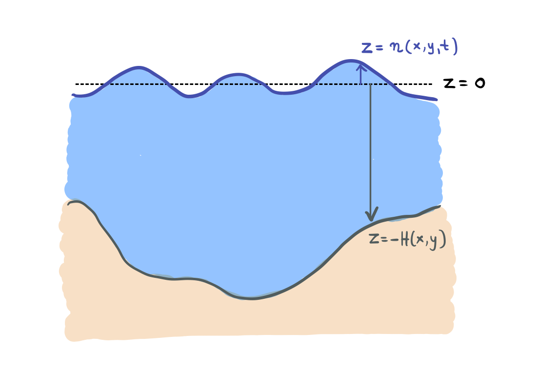
Mass conservation and free surface evolution equation

The mass conservation equation is

Given the horizontal flow we use the above to diagnose the vertical velocity . We integrate the mass conservation equation from the bottom of the fluid (where  ) up to depth and recover .

The free surface displacement satisfies the linearized kinematic boundary condition at the surface

The momentum conservation equation

The equations governing the conservation of momentum in a rotating fluid, including buoyancy via the Boussinesq approximation are

where the is buoyancy, is the hydrostatic kinematic stress tensor, denotes an internal forcing of the horizontal flow ,    is the three-dimensional flow, is kinematic pressure, is the free-surface displacement, and is the Coriolis parameter, or the background vorticity associated with the specified rate of rotation of the frame of reference.

We can recast the advection term   above in vector-invariant form as:

with    the vertical component of the relative vorticity. The vector-invariant form is used with curvilinear grids, like LatitudeLongitudeGrid or OrthogonalSphericalShellGrid.

The hydrostatic approximation above comes about as the dominant balance of terms in the Navier-Stokes vertical momentum equation under the Boussinesq approximation.

The terms that appear on the right-hand side of the momentum conservation equation are (in order):

• momentum advection: ,

• Coriolis:  ,

• baroclinic kinematic pressure gradient: ,

• barotropic kinematic pressure gradient: ,

• molecular or turbulence viscous stress:  , and

• an arbitrary internal source of momentum: .

The tracer conservation equation

The conservation law for tracers is

where is the diffusive flux of and is an arbitrary source term. An arbitrary tracers are permitted and thus an arbitrary number of tracer equations can be solved simultaneously alongside with the momentum equations.

From left to right, the terms that appear on the right-hand side of the tracer conservation equation are

• tracer advection:  ,

• molecular or turbulent diffusion:  , and

• an arbitrary internal source of tracer: .

Vertical coordinates

We can use either ZCoordinate, that is height coordinate, or the ZStarCoordinate generalized vertical coordinate.

The ZStarCoordinate vertical coordinate conserves tracers and volume with the grid following the evolution of the free surface in the domain (Adcroft and Campin, 2004).

In terms of the notation in the Generalized vertical coordinates section, for a ZCoordinate we have that

and the specific thickness is   .

The ZStarCoordinate generalized vertical coordinate is often denoted as (zee-star), i.e.,

where is the free surface and    is the bottom of the domain.

Note that in both depth and coordinates, the bottom boundary is the same    . On the other hand, while in depth coordinates the upper boundary   changes with time, but in coordinates is fixed to  .

The ZStarCoordinate definition implies a specific thickness

All the equations transformed in -coordinates are described in the Generalized vertical coordinates section.

For the specific choice of ZStarCoordinate coordinate , the identically vanishes and thus the horizontal gradient of the free surface remain unchanged under vertical coordinate transformation, i.e.,

An example of how the vertical coordinate surfaces differ for ZCoordinate and the time-varying ZStarCoordinate coordinate is shown below.

using CairoMakie

Lx, Lz = 1e3, 25 # m

x = range(-Lx/2, stop=Lx/2, length=200)

σ = Lx/15 # a horizontal length scale

# bottom, H(x)
x₀, h₀ = -Lx/3,  15 # m
slope = @. h₀ * (1 + tanh(-(x - x₀) / σ)) / 2
x₀, h₀ = Lx/3, 6 # m
mountain = @. h₀ * sech((x - x₀) / σ)^2
H = @. Lz - slope - mountain

# free surface, η(x)
x₀ = -Lx/8
η₀ = 2.5 # m
t = Observable(0.0)
η = @lift @. -η₀ * ((x - x₀)^2 / σ^2 - 1) * exp(-(x - x₀)^2 / 2σ^2) * cos(2π * $t)

fig = Figure(size=(1000, 400))
axis_kwargs = (titlesize = 20, xlabel = "x", ygridvisible = false)
ax1 = Axis(fig[1, 1]; title="ZCoordinate", ylabel="z", axis_kwargs...)
ax2 = Axis(fig[1, 2]; title="ZStarCoordinate", axis_kwargs...)

for ax in (ax1, ax2)
    band!(ax, x, -H, η, color = (:dodgerblue, 0.5))
    band!(ax, x, -1.1 * Lz, -H, color = (:orange, 0.2))
    lines!(ax, x,  η, linewidth=5, color=:darkblue)
    lines!(ax, x, -H, linewidth=5, color=:darkgrey)
end

for r in range(-Lz, stop=0, length=6)
    # ZCoordinate
    z = r * ones(size(x))
    lines!(ax1, x, z, color=:crimson, linestyle=:dash)

    # ZStarCoordinate
    z = lift(η) do η_val
        @. r * (H + η_val) / H + η_val
    end
    lines!(ax2, x, z, color=:crimson, linestyle=:dash)
end

Nt = 50
times = 0:1/Nt:1-1/Nt # one period of cos(2πt)
CairoMakie.record(fig, "z-zstar.gif", times, framerate=12) do val
    t[] = val
end

Near the top, the surfaces of ZStarCoordinate mimic the free surface. Further away from the fluid's surface, the surfaces of ZStarCoordinate resemble more surfaces of constant depth ZCoordinate.