Ensemble Kalman Sampling

What Is It and What Does It Do?

The Ensemble Kalman Sampler (EKS) (Garbuno-Inigo et al, 2020, Cleary et al, 2020, and it's variant Affine-invariant interacting Langevin Dynamics (ALDI) Garbuno-Inigo et al, 2020) are derivative-free tools for approximate Bayesian inference. They does so by approximately sampling from the posterior distribution. That is, EKS provides both point estimation (through the mean of the final ensemble) and uncertainty quantification (through the covariance of the final ensemble), this is in contrast to EKI, which only provides point estimation.

The EKS algorithm, viewed affine invariant system of interacting particles (Garbuno-Inigo et al, 2020) and ALDI differs from EKS by a finite-sample correction is introduced to overcome its computational finite-sample implementation. Both of these variants are provided through the Sampler process in our the toolbox - by default we construct this improved ALDI variant.

While there are noisy variants of the standard EKI, EKS differs from them in its noise structure (as its noise is added in parameter space, not in data space), and its update rule explicitly accounts for the prior (rather than having it enter through initialization). The approximatiom of the posterior through EKS typically needs more iterations than EKI to converge to a suitable solution, and to help we provide an adaptive learning rate scheduler EKSStableScheduler() and a semi-implicit formulation to help maintain a stable interacting particle system. However, the posterior approximation through EKS is obtained with far less computational effort than a typical Markov Chain Monte Carlo (MCMC) like Metropolis-Hastings, though it will provide Gaussian-like uncertainty.

Problem Formulation

The data $y$ and parameter vector $\theta$ are assumed to be related according to:

\[ y = \mathcal{G}(\theta) + \eta \,,\]

where $\mathcal{G}: \mathbb{R}^p \rightarrow \mathbb{R}^d$ denotes the forward map, $y \in \mathbb{R}^d$ is the vector of observations, and $\eta$ is the observational noise, which is assumed to be drawn from a $d$-dimensional Gaussian with distribution $\mathcal{N}(0, \Gamma_y)$. The objective of the inverse problem is to compute the unknown parameters $\theta$ given the observations $y$, the known forward map $\mathcal{G}$, and noise characteristics $\eta$ of the process.

Ensemble Kalman Sampling Algorithm

The EKS is based on the following update equation for the parameter vector $\theta^{(j)}_n$ of ensemble member $j$ at the $n$-iteration:

\[\begin{aligned} \theta_{n+1}^{(*, j)} &= \theta_{n}^{(j)} - \dfrac{\Delta t_n}{J}\sum_{k=1}^J\langle \mathcal{G}(\theta_n^{(k)}) - \bar{\mathcal{G}}_n, \Gamma_y^{-1}(\mathcal{G}(\theta_n^{(j)}) - y) \rangle \theta_{n}^{(k)} + \frac{d+1}{J} \left(\theta_{n}^{(j)} - \bar \theta_n \right) - \Delta t_n \mathsf{C}(\Theta_n) \Gamma_{\theta}^{-1} \theta_{n + 1}^{(*, j)} \,, \\ \theta_{n + 1}^{j} &= \theta_{n+1}^{(*, j)} + \sqrt{2 \Delta t_n \mathsf{C}(\Theta_n)} \xi_n^{j} \,, \end{aligned}\]

where the subscript $n=1, \dots, N_{\text{it}}$ indicates the iteration, $J$ is the ensemble size (i.e., the number of particles in the ensemble), $\Delta t_n$ is an internal adaptive time step (thus no need for the user to specify), $\Gamma_{\theta}$ is the prior covariance, and $\xi_n^{(j)} \sim \mathcal{N}(0, \mathrm{I}_p)$. $\bar{\mathcal{G}}_n$ is the ensemble mean of the forward map $\mathcal{G}(\theta)$,

\[\bar{\mathcal{G}}_n = \dfrac{1}{J}\sum_{k=1}^J\mathcal{G}(\theta_n^{(k)})\,.\]

The $p \times p$ matrix $\mathsf{C}(\Theta_n)$, where $\Theta_n = \left\{\theta^{(j)}_n\right\}_{j=1}^{J}$ is the set of all ensemble particles in the $n$-th iteration, denotes the empirical covariance between particles

\[\mathsf{C}(\Theta_n) = \frac{1}{J} \sum_{k=1}^J (\theta^{(k)}_n - \bar{\theta}_n) \otimes (\theta^{(k)}_n - \bar{\theta}_n)\,,\]

where $\bar{\theta}_n$ is the ensemble mean of the particles,

\[\bar{\theta}_n = \dfrac{1}{J}\sum_{k=1}^J\theta^{(k)}_n \,.\]

Constructing the Forward Map

At the core of the forward map $\mathcal{G}$ is the dynamical model $\Psi:\mathbb{R}^p \rightarrow \mathbb{R}^o$ (running $\Psi$ is usually where the computational heavy-lifting is done), but the map $\mathcal{G}$ may include additional components such as a transformation of the (unbounded) parameters $\theta$ to a constrained domain the dynamical model can work with, or some post-processing of the output of $\Psi$ to generate the observations. For example, $\mathcal{G}$ may take the following form:

\[\mathcal{G} = \mathcal{H} \circ \Psi \circ \mathcal{T}^{-1},\]

where $\mathcal{H}:\mathbb{R}^o \rightarrow \mathbb{R}^d$ is the observation map and $\mathcal{T}$ is the transformation from the constrained to the unconstrained parameter space, such that $\mathcal{T}(\phi)=\theta$. A family of standard transformations and their inverses are available in the ParameterDistributions module.

How to Construct an Ensemble Kalman Sampler

An EKS object can be created using the EnsembleKalmanProcess constructor by specifying the Sampler type. The constructor takes an argument, the prior. The following example shows how an EKS object is instantiated. An observation (y) and the covariance of the observational noise (obs_cov) are assumed to be defined previously in the code.

using EnsembleKalmanProcesses # for `construct_initial_ensemble`,`EnsembleKalmanProcess`
using EnsembleKalmanProcesses.ParameterDistributions  # for `ParameterDistribution`

# Construct prior (see `ParameterDistributions.jl` docs)
prior = ParameterDistribution(...)


# Construct initial ensemble
N_ens = 20  # ensemble size
initial_ensemble = construct_initial_ensemble(prior, N_ens)

# Construct ensemble Kalman process
eksobj = EnsembleKalmanProcess(initial_ensemble, y, obs_noise_cov, Sampler(prior))

One can also build the original EKS variant (not ALDI), with the sampler_type keyword

Sampler(prior, sampler_type="eks")

Updating the ensemble

Once the EKS object eksobj has been initialized, the initial ensemble of particles is iteratively updated by the update_ensemble! function, which takes as arguments the eksobj and the evaluations of the forward model at each member of the current ensemble. In the following example, the forward map G maps a parameter to the corresponding data – this is done for each parameter in the ensemble, such that the resulting g_ens is of size d x N_ens. The update_ensemble! function then stores the updated ensemble as well as the evaluations of the forward map in eksobj.

A typical use of the update_ensemble! function given the EKS object eksobj, the dynamical model Ψ, and the observation map H (the latter two are assumed to be defined elsewhere, e.g. in a separate module) may look as follows:

# Given:
# Ψ (some black box simulator)
# H (some observation of the simulator output)
# prior (prior distribution and parameter constraints)

N_iter = 100 # Number of iterations

for n in 1:N_iter
    ϕ_n = get_ϕ_final(prior, eksobj) # Get current ensemble in constrained "ϕ"-space
    G_n = [H(Ψ(ϕ_n[:, i])) for i in 1:J]  # Evaluate forward map
    g_ens = hcat(G_n...)  # Reformat into `d x N_ens` matrix
    update_ensemble!(eksobj, g_ens) # Update ensemble
end

Solution

The solution of the EKS algorithm is an approximate Gaussian distribution whose mean (u_post) and covariance (Γ_post) can be extracted from the ''final ensemble'' (i.e., after the last iteration). The sample mean of the last ensemble is also the "optimal" parameter (u_optim) for the given calibration problem. These statistics can be accessed as follows:

# mean of the Gaussian distribution, the optimal parameter in computational u-space
u_post = get_u_mean_final(eksobj)
# (empirical) covariance of the Gaussian distribution in computational u-space
Γ_post = get_u_cov_final(eksobj)

# constrained samples in physical space (prior contains the physical encoding)
ϕ = get_ϕ_final(prior, eksobj)

To obtain new samples of this approximate posterior in the constrained space, we first sample the distribution, then transform using the constraints contained within the prior

using Random, Distributions

ten_post_samples = rand(MvNormal(u_post,Γ_post), 10)
ten_post_samples_phys = transform_unconstrained_to_constrained(prior, ten_post_samples) # the optimal physical parameter value

Quick comparison of samplers

From examples/LossMinimization/loss_minimization_finite_vs_infinite_ekp.jl. Quick comparison between three samplers ALDI, EKS, and GNKI, taken attheir current defaults. We also plot of error vs spread over the iterations

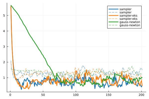
• In black: Prior and posterior distribution contours
• error (solid) is defined by $\frac{1}{N_{ens}}\sum^{N_{ens}}_{i=1} \| \theta_i - \theta^* \|^2$ where $\theta_i$ are ensemble members and $\theta^*$ is the true value used to create the observed data.
• spread (dashed) is defined by $\frac{1}{N_{ens}}\sum^{N_{ens}}_{i=1} \| \theta_i - \bar{\theta} \|^2$ where $\theta_i$ are ensemble members and $\bar{\theta}$ is the mean over these members.

We see the ensemble does not collapse and samples the posterior distribution. The statistics over long times of these methods are statistically the same, though the EKS/ALDI variant has faster convergence than GNKI.