Learning the permeability field in a Darcy flow

In this example, we illustrate a simple function learning problem. We are presented with an unknown field that is discretized with a finite-dimensional approximation (e.g. spatial discretization). When learning this field, if one represents each pointwise value at a gridpoint as a parameter, increasing the spatial resolution leads to increasingly high dimensional learning problems, thus giving poor computational scaling and increasingly ill-posed inverse problems from fixed data. If instead, we treat the approximation as a discretized function living in a function space, then one can learn coefficients of a basis of this function space. Since it is commonly the case that functions have relatively low effective dimension in this space, the dependence on the spatial discretization only arises in discretization error, which vanishes as resolution is increased.

We will solve for an unknown permeability field $\kappa$ governing the pressure field $h$ of a Darcy flow on a square 2D domain $\Omega$. The pressure obeys the elliptic equation

\[-\nabla \cdot (\kappa \nabla h) = f, \qquad h = 0 \text{ on } \partial\Omega,\]

for a given source term $f$. To learn about the permeability we shall take few pointwise measurements of the solved pressure field within the domain. The forward solver is a simple finite difference scheme taken and modified from code here.

Walkthrough of the code

First we load standard packages,

using LinearAlgebra
using Distributions
using Random
using JLD2

the package to define the function distributions,

import GaussianRandomFields # we wrap this so we don't want to use "using"
const GRF = GaussianRandomFields

GaussianRandomFields

and finally the EKP packages.

using EnsembleKalmanProcesses
using EnsembleKalmanProcesses.ParameterDistributions
const EKP = EnsembleKalmanProcesses

EnsembleKalmanProcesses

We include the forward solver here. (The path is resolved from the package directory so that this also works from within the documentation build.)

include(joinpath(pkgdir(EKP), "examples", "Darcy", "GModel.jl"))

compute_obs (generic function with 1 method)

Then link some outputs for figures and saved data, and we load Plots.jl.

fig_save_directory = joinpath(@__DIR__, "output")
data_save_directory = joinpath(@__DIR__, "output")
mkpath(fig_save_directory)
mkpath(data_save_directory)

using Plots

Set a random seed.

seed = 100234
rng = Random.MersenneTwister(seed)

Define the spatial domain and discretization.

dim = 2
N, L = 80, 1.0
pts_per_dim = LinRange(0, L, N)
obs_ΔN = 10

To provide a simple test case, we assume that the true function parameter is a particular sample from the function space we set up to define our prior. We choose a value of the truth that doesn't have a vanishingly small probability under the prior defined by a probability distribution over functions; taken to be a family of Gaussian Random Fields (GRF). This function distribution is characterized by a covariance function - here a Matern kernel which assumes a level of smoothness over the samples from the distribution - and an appropriate representation - here based on the Karhunen-Loeve expansion (similar to an eigenvalue-eigenfunction expansion). The representation is truncated to a finite number of coefficients, the degrees of freedom (dofs), which define the effective dimension of the learning problem that is decoupled from the spatial discretization. Larger dofs may be required to represent multiscale functions, but come at an increased dimension of the parameter space and therefore a typical increase in cost and difficulty of the learning problem. For more details see GaussianRandomFields.jl.

smoothness = 1.0
corr_length = 0.25
dofs = 50

grf = GRF.GaussianRandomField(
    GRF.CovarianceFunction(dim, GRF.Matern(smoothness, corr_length)),
    GRF.KarhunenLoeve(dofs),
    pts_per_dim,
    pts_per_dim,
)

We define a wrapper around the GRF, and as the permeability field must be positive we introduce a domain constraint into the function distribution. Henceforth, the GRF is interfaced in the same manner as any other parameter distribution.

pkg = GRFJL()
distribution = GaussianRandomFieldInterface(grf, pkg) # our wrapper from EKP
domain_constraint = bounded_below(0) # make κ positive
pd = ParameterDistribution(Dict("distribution" => distribution, "name" => "kappa", "constraint" => domain_constraint)) # the fully constrained parameter distribution

ParameterDistribution with 1 entry
  'kappa': GaussianRandomFieldInterface (GRFJL, 1 dofs) [1 constraint]

Now we have a function distribution, we sample a reasonably high-probability value from this distribution as a true value (here all degrees of freedom are set to $u_{\mathrm{true}} = -1.5$); this choice is arbitrary, up to not having a vanishingly small mass under the prior. We use the EKP transform function to build the corresponding instance of the $\kappa_{\mathrm{true}}$.

u_true = -1.5 * ones(dofs, 1) # the truth parameter
κ_true = transform_unconstrained_to_constrained(pd, u_true) # builds and constrains the function.
κ_true = reshape(κ_true, N, N)

Now we generate the data sample for the truth in a perfect model setting by evaluating the model here, and observing the pressure field at a few subsampled points in each dimension (here obs_ΔN, samples every 10 points in each dimension, leading to a $7 \times 7$ observation grid), and we assume 5% additive observational noise on the measurements.

darcy = Setup_Param(pts_per_dim, obs_ΔN, κ_true)
println(" Number of observation points: $(darcy.N_y)")
h_2d_true = solve_Darcy_2D(darcy, κ_true)
y_noiseless = compute_obs(darcy, h_2d_true)
obs_noise_cov = 0.05^2 * I(length(y_noiseless)) * (maximum(y_noiseless) - minimum(y_noiseless))
truth_sample = vec(y_noiseless + rand(rng, MvNormal(zeros(length(y_noiseless)), obs_noise_cov)))

 Number of observation points: 49

Now we set up the Bayesian inversion algorithm. The prior we have already defined to construct our truth.

prior = pd

We define some algorithm parameters, here we take ensemble members larger than the dimension of the parameter space to ensure a full rank ensemble covariance.

N_ens = 50 # number of ensemble members
N_iter = 20 # number of EKI iterations

We sample the initial ensemble from the prior, and create the EKP object as an EKI algorithm using the Inversion() keyword.

initial_params = construct_initial_ensemble(rng, prior, N_ens)
ekiobj = EKP.EnsembleKalmanProcess(initial_params, truth_sample, obs_noise_cov, Inversion())

┌ Warning: For 50 parameters, the recommended minimum ensemble size (`N_ens`) is 100. Got `N_ens` = 50`.
└ @ EnsembleKalmanProcesses ~/work/EnsembleKalmanProcesses.jl/EnsembleKalmanProcesses.jl/src/EnsembleKalmanProcess.jl:265

We perform the inversion loop. Remember that within calls to get_ϕ_final the EKP transformations are applied, thus the ensemble that is returned will be the positively-bounded permeability field evaluated at all the discretization points. We also check for termination criteria (from the default DataMisfitController scheduler), and break the loop if the criteria are exceeded - on termination, the update is not performed.

println("Begin inversion")
err = []
final_it = [N_iter]
for i in 1:N_iter
    params_i = get_ϕ_final(prior, ekiobj)
    g_ens = run_G_ensemble(darcy, params_i)
    terminate = EKP.update_ensemble!(ekiobj, g_ens)
    push!(err, get_error(ekiobj)[end]) #mean((params_true - mean(params_i,dims=2)).^2)
    println("Iteration: " * string(i) * ", Error: " * string(err[i]))
    if !isnothing(terminate)
        final_it[1] = i - 1
        break
    end
end
n_iter = final_it[1]

Begin inversion
Iteration: 1, Error: 20178.451602552355
Iteration: 2, Error: 9094.864563369367
Iteration: 3, Error: 6959.958347953093
Iteration: 4, Error: 2839.5795555496597
Iteration: 5, Error: 1278.3476407970531
Iteration: 6, Error: 575.498465602039
Iteration: 7, Error: 284.4023383772008
Iteration: 8, Error: 171.43711780560832
Iteration: 9, Error: 120.12667046852165
Iteration: 10, Error: 86.10855806309337
Iteration: 11, Error: 67.19816956675369
Iteration: 12, Error: 67.10980101598423
Iteration: 13, Error: 71.59839061789823
Iteration: 14, Error: 76.23458343986857
Iteration: 15, Error: 78.40690680808882
Iteration: 16, Error: 77.76370631281779
Iteration: 17, Error: 75.92298553044411
Iteration: 18, Error: 72.75098445016397
Iteration: 19, Error: 68.71526672203433
Iteration: 20, Error: 64.42993956295822

Inversion results

We plot first the prior ensemble mean and pointwise variance of the permeability field, and also the pressure field solved with the ensemble mean. Each ensemble member is stored as a column and therefore for uses such as plotting one needs to reshape to the desired dimension.

gr(size = (1500, 400), legend = false)

prior_κ_ens = get_ϕ(prior, ekiobj, 1)
κ_ens_mean = reshape(mean(prior_κ_ens, dims = 2), N, N)
p1 = contour(pts_per_dim, pts_per_dim, κ_ens_mean', fill = true, levels = 15, title = "kappa mean", colorbar = true)
κ_ens_ptw_var = reshape(var(prior_κ_ens, dims = 2), N, N)
p2 = contour(pts_per_dim, pts_per_dim, κ_ens_ptw_var', fill = true, levels = 15, title = "kappa var", colorbar = true)
h_2d = solve_Darcy_2D(darcy, κ_ens_mean)
p3 = contour(pts_per_dim, pts_per_dim, h_2d', fill = true, levels = 15, title = "pressure", colorbar = true)
l = @layout [a b c]
plt = plot(p1, p2, p3, layout = l)
plt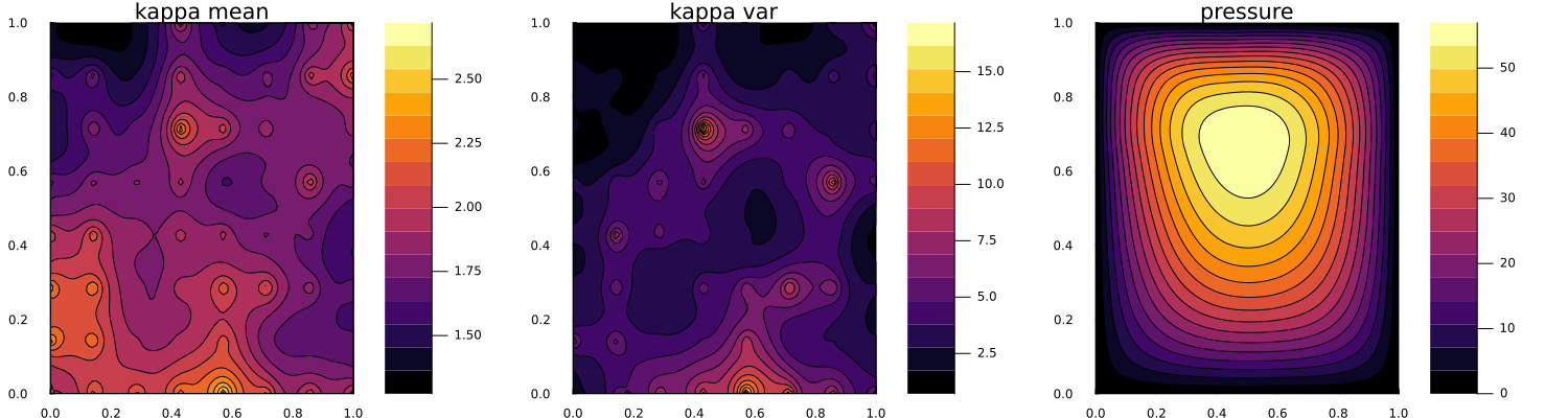

Now we plot the final ensemble mean and pointwise variance of the permeability field, and also the pressure field solved with the ensemble mean.

final_κ_ens = get_ϕ_final(prior, ekiobj) # the `ϕ` indicates that the `params_i` are in the constrained space
κ_ens_mean = reshape(mean(final_κ_ens, dims = 2), N, N)
p1 = contour(pts_per_dim, pts_per_dim, κ_ens_mean', fill = true, levels = 15, title = "kappa mean", colorbar = true)
κ_ens_ptw_var = reshape(var(final_κ_ens, dims = 2), N, N)
p2 = contour(pts_per_dim, pts_per_dim, κ_ens_ptw_var', fill = true, levels = 15, title = "kappa var", colorbar = true)
h_2d = solve_Darcy_2D(darcy, κ_ens_mean)
p3 = contour(pts_per_dim, pts_per_dim, h_2d', fill = true, levels = 15, title = "pressure", colorbar = true)
l = @layout [a b c]
plt = plot(p1, p2, p3; layout = l)
plt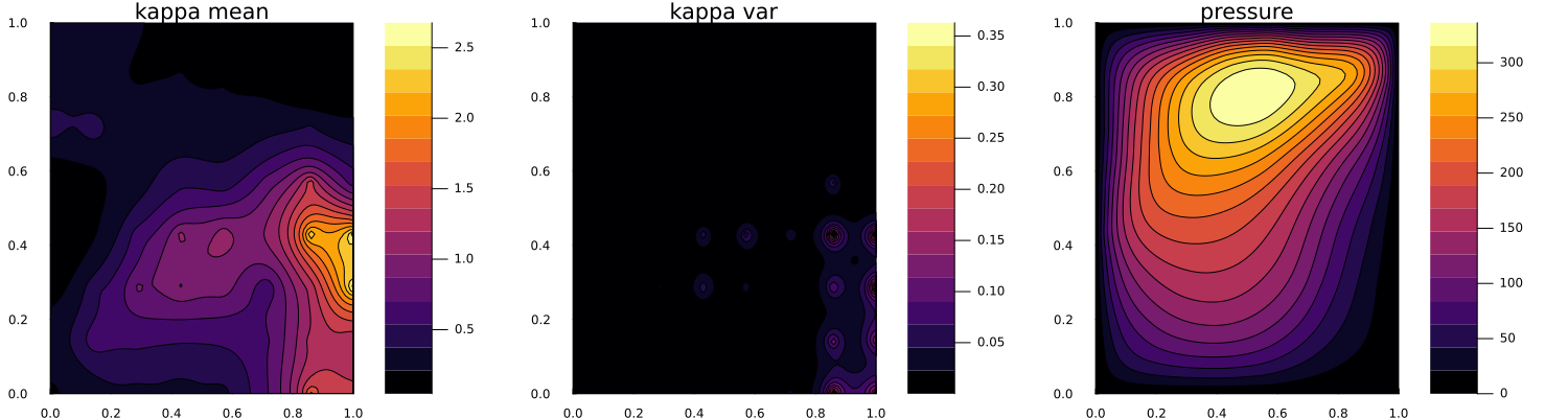

We can compare this with the true permeability and pressure field.

gr(size = (1000, 400), legend = false)
p1 = contour(pts_per_dim, pts_per_dim, κ_true', fill = true, levels = 15, title = "kappa true", colorbar = true)
p2 = contour(pts_per_dim, pts_per_dim, h_2d_true', fill = true, levels = 15, title = "pressure true", colorbar = true)
l = @layout [a b]
plt = plot(p1, p2, layout = l)
plt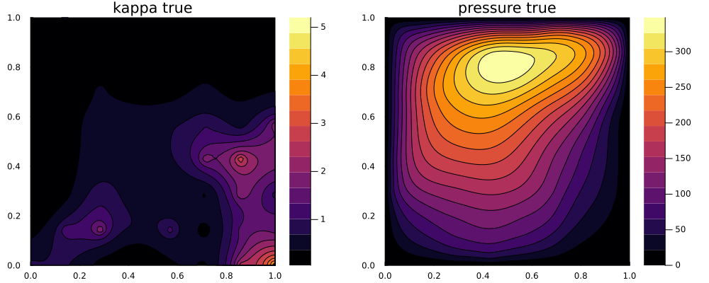

Finally the data is saved.

u_stored = get_u(ekiobj, return_array = false)
g_stored = get_g(ekiobj, return_array = false)
@save joinpath(data_save_directory, "parameter_storage.jld2") u_stored
@save joinpath(data_save_directory, "data_storage.jld2") g_stored

This page was generated using Literate.jl.