Convergence Tests

Convergence tests are implemented in /validation/convergence_tests and range from zero-dimensional time-stepper tests to two-dimensional integration tests that involve non-trivial pressure fields, advection, and diffusion.

For all tests except point exponential decay, we use the $L_1$ norm,

\[ L_1 \equiv \frac{\mathrm{mean} | \phi_\mathrm{sim} - \phi_\mathrm{exact} |}{\mathrm{mean} | \phi_\mathrm{exact} |}\]

and $L_\infty$ norm,

\[ L_\infty \equiv \frac{\max | \phi_\mathrm{sim} - \phi_\mathrm{exact} |}{\max | \phi_\mathrm{exact} |} \, ,\]

to compare simulated fields, $\phi_\mathrm{sim}$, with exact, analytically-derived solutions $\phi_\mathrm{exact}$. The field $\phi$ may be a tracer field or a velocity field.

Point Exponential Decay

This test analyzes time-stepper convergence by simulating the zero-dimensional, or spatially-uniform equation

\[ \partial_t c = - c \, ,\]

with the initial condition $c = 1$, which has the analytical solution $c = \mathrm{e}^{-t}$.

We find the expected first-order convergence with decreasing time-step $\Delta t$ using our first-order accurate, "modified second-order" Adams-Bashforth time-stepping method:

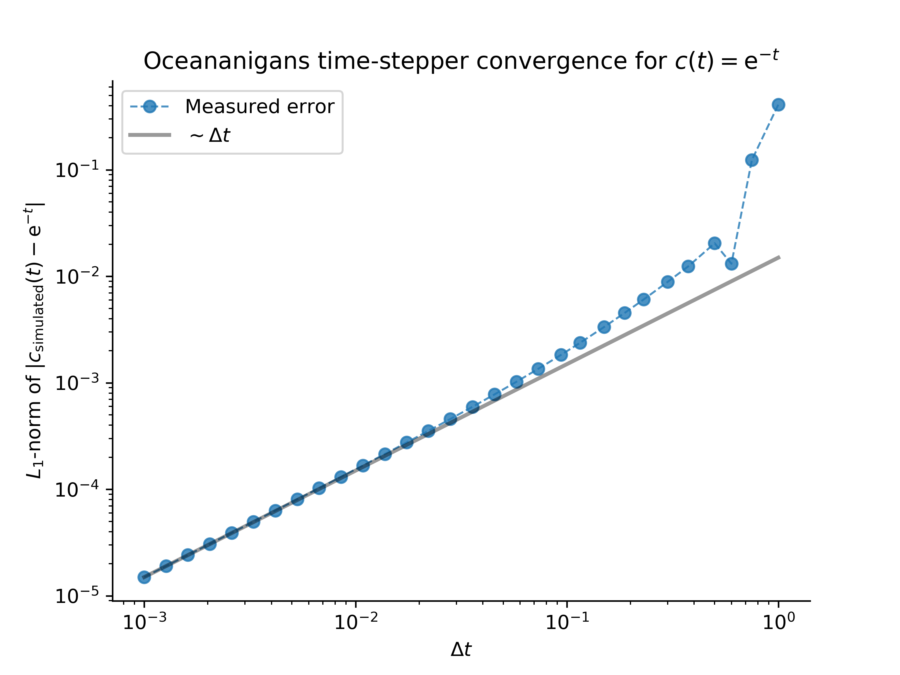
This result validates the correctness of the Oceananigans implementation of Adams-Bashforth time-stepping.

One-dimensional advection and diffusion of a Gaussian

This and the following tests focus on convergence with grid spacing, $\Delta x$.

In one dimension with constant diffusivity $\kappa$ and in the presence of a constant velocity $U$, a Gaussian evolves according to

\[ c = \frac{\mathrm{e}^{- (x - U t)^2 / 4 \kappa t}}{\sqrt{4 \pi \kappa t}} \, .\]

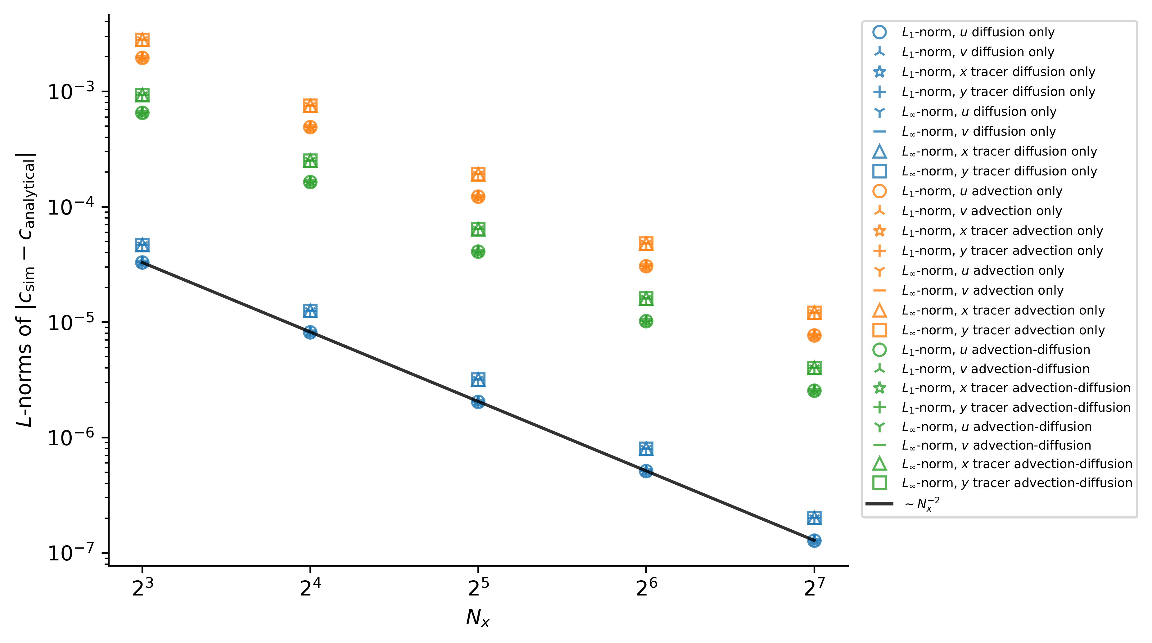
For this test we take the initial time as $t=t_0$. We simulate this problem with advection and diffusion, as well as with $U=0$ and thus diffusion only, as well as with $\kappa \approx 0$ and thus "advection only". The solutions are

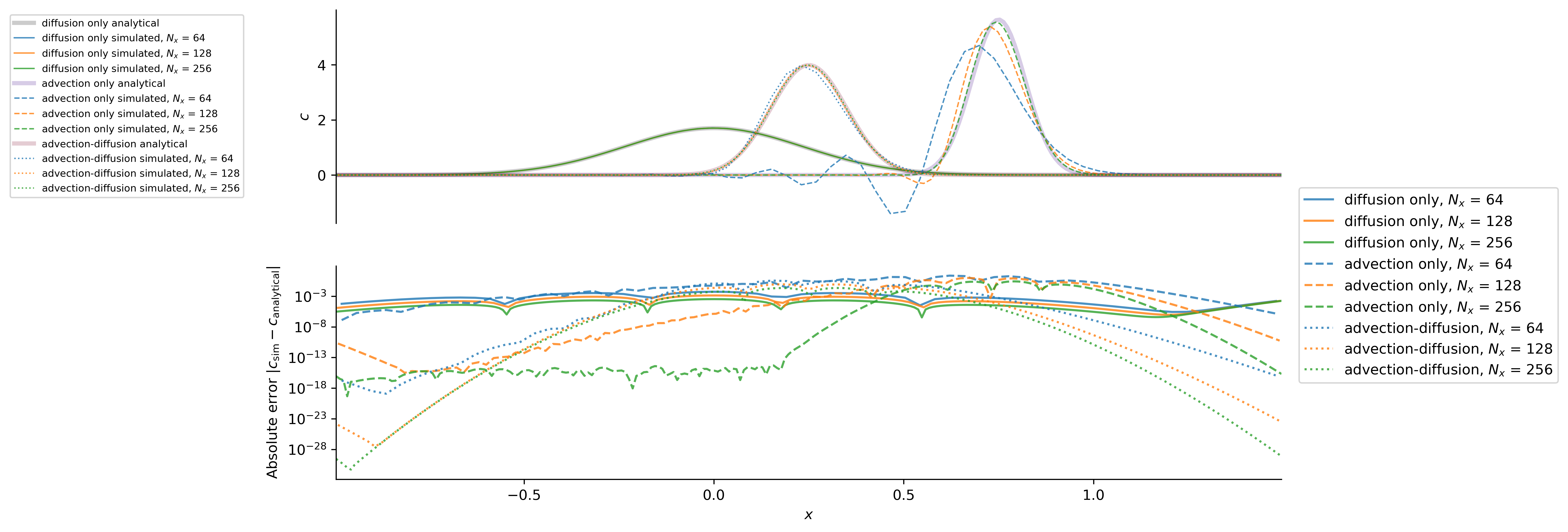
which exhibit the expected second-order convergence with $\Delta x^2 \propto 1 / N_x^2$:

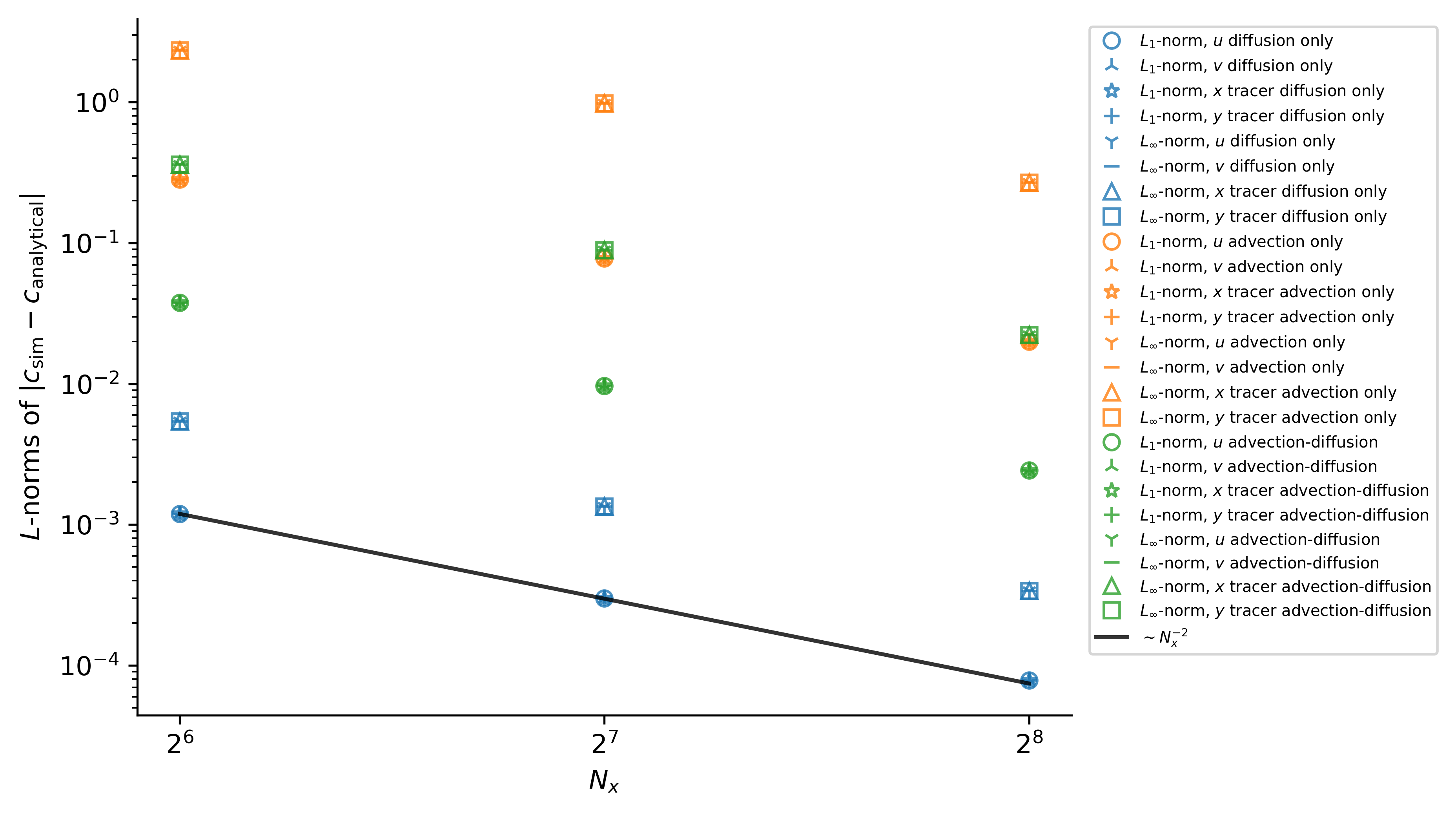
These results validate the correctness of time-stepping, constant diffusivity operators, and advection operators.

One-dimensional advection and diffusion of a cosine

In one dimension with constant diffusivity $\kappa$ and in the presence of a constant velocity $U$, a cosine evolves according to

\[ c = \mathrm{e}^{-\kappa t} \cos (x - U t) \, .\]

The solutions are

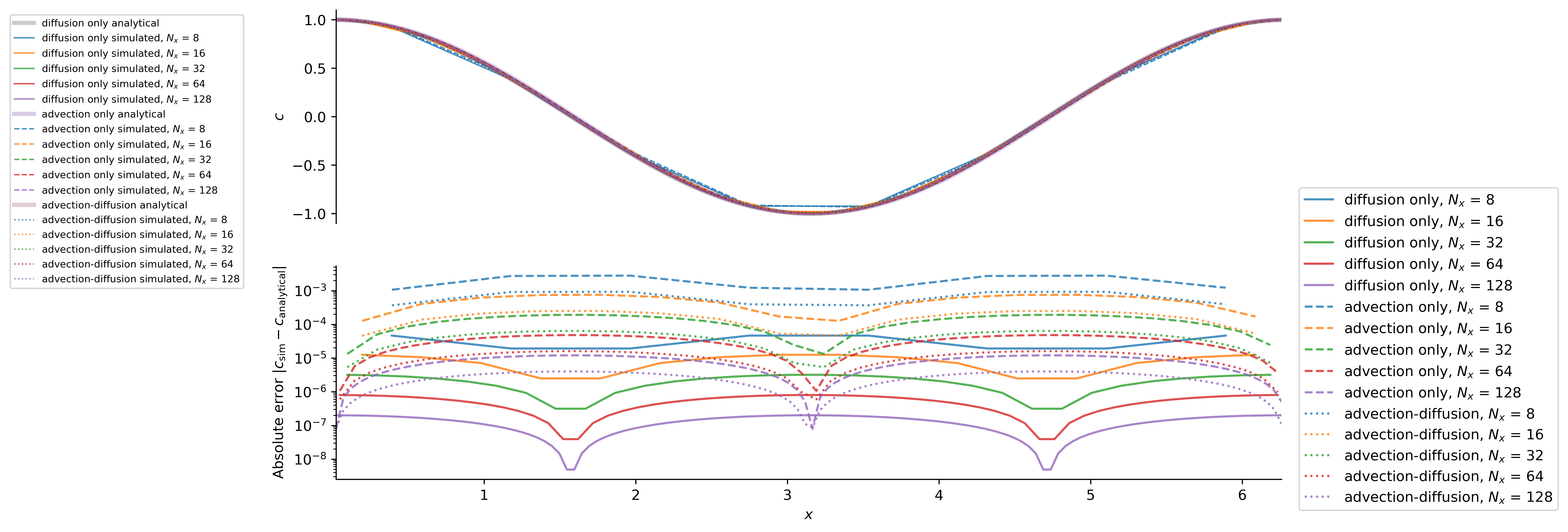
which exhibit the expected second-order convergence with $\Delta x^2 \propto 1 / N_x^2$:

These results validate the correctness of time-stepping, constant diffusivity operators, and advection operators.

Two-dimensional diffusion

With zero velocity field and constant diffusivity $\kappa$, the tracer field

\[ c(x, y, t=0) = \cos(x) \cos(y) \, ,\]

decays according to

\[ c(x, y, t) = \mathrm{e}^{-2 \kappa t} \cos(x) \cos(y) \, ,\]

with either periodic boundary conditions, or insulating boundary conditions in either $x$ or $y$.

The expected convergence with $\Delta x^2 \propto 1 / N_x^2$ is observed:

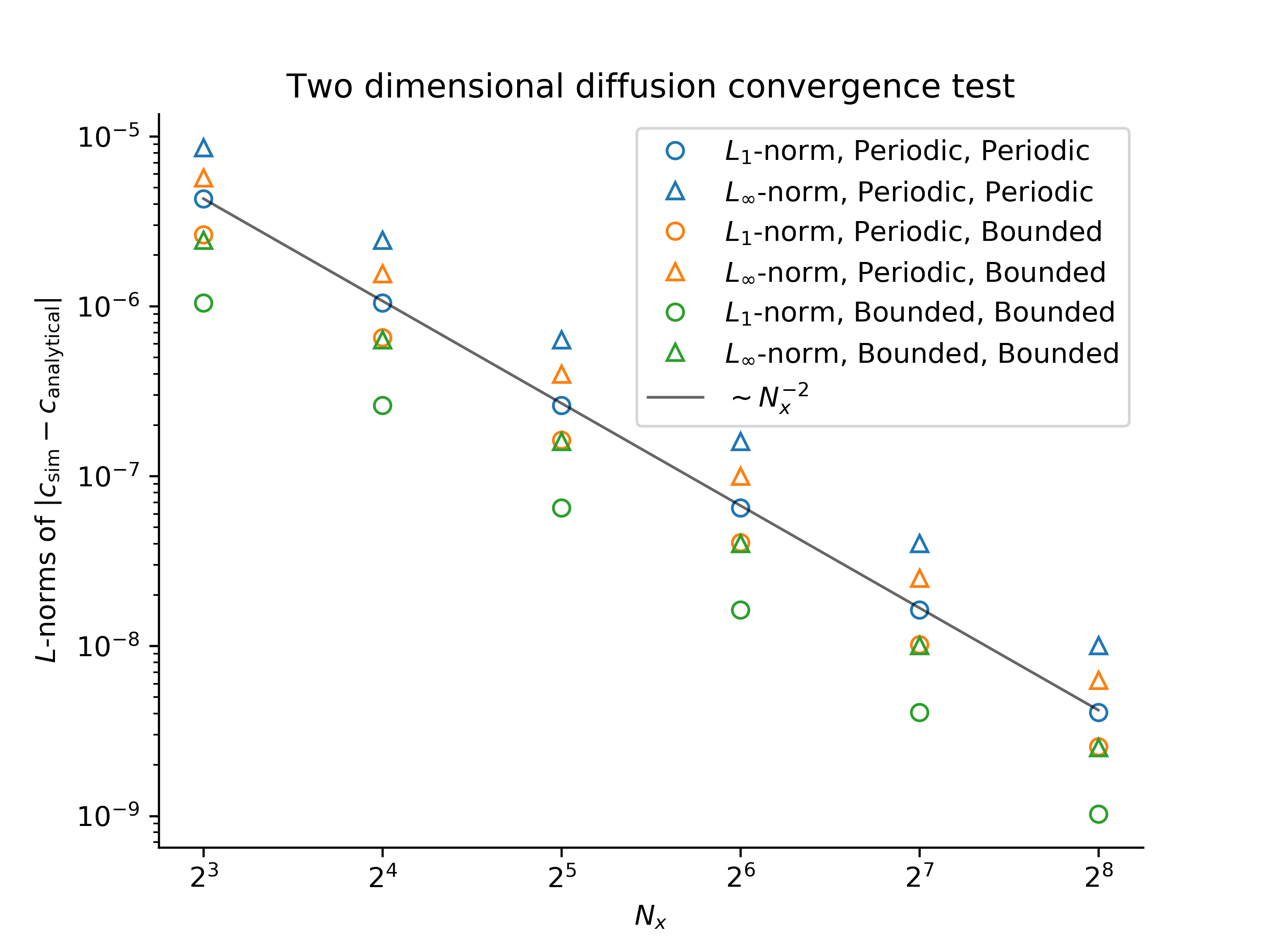
This validates the correctness of multi-dimensional diffusion operators.

Decaying, advected Taylor-Green vortex

The velocity field

\[\begin{align} u(x, y, t) & = U + \mathrm{e}^{-t} \cos(x - U t) \sin(y) \, , \\ v(x, y, t) & = - \mathrm{e}^{-t} \sin(x - U t) \cos(y) \, , \end{align}\]

is a solution to the Navier-Stokes equations with viscosity $\nu = 1$.

The expected convergence with spatial resolution is observed:

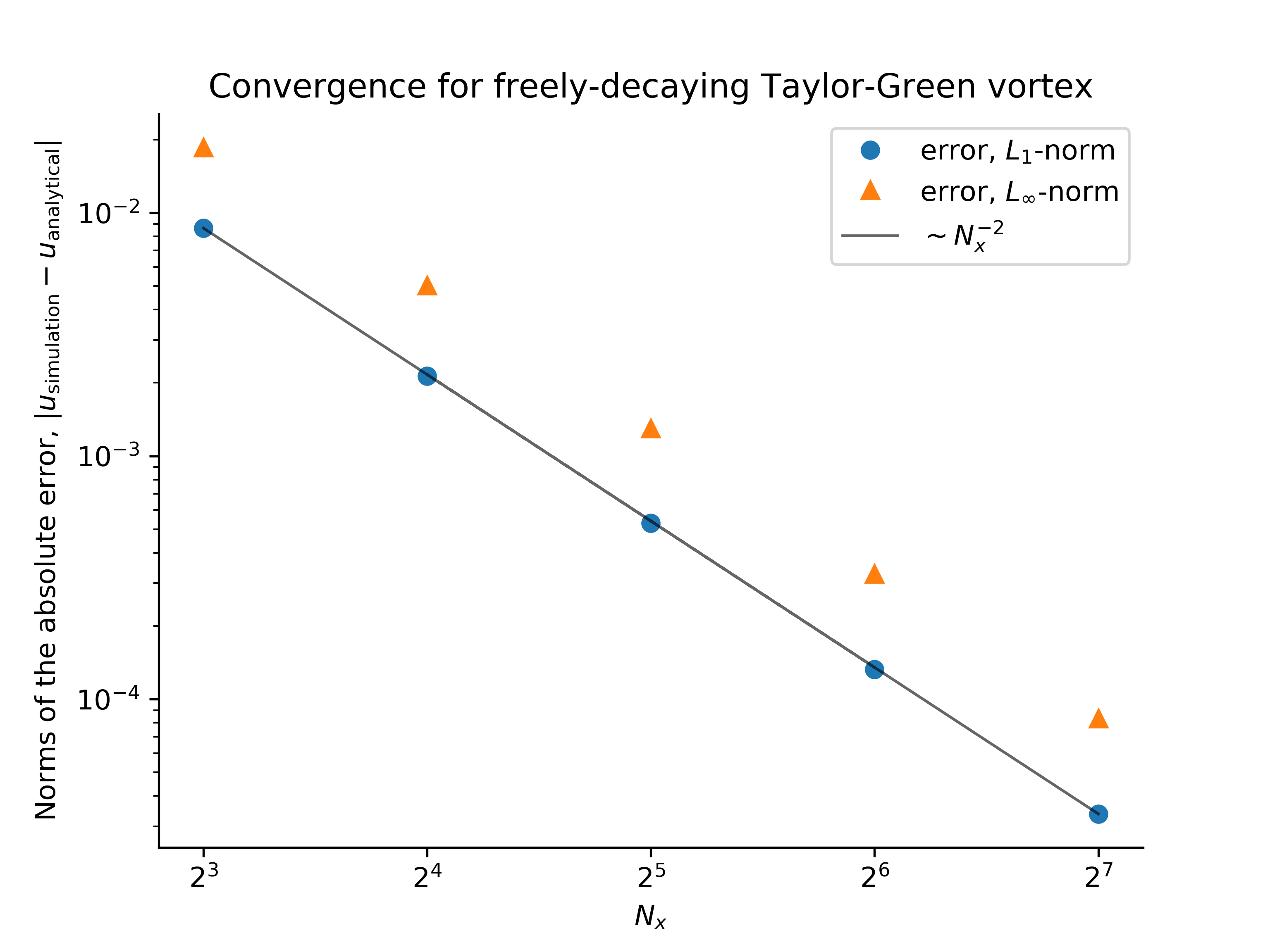
This validates the correctness of the advection and diffusion of a velocity field.

Forced two-dimensional flows

We introduce two convergence tests associated with forced flows in domains that are bounded in $y$, and periodic in $x$ with no tracers.

Note: in this section, subscripts are used to denote derivatives to make reading and typing equations easier.

In a two-dimensional flow in $(x, y)$, the velocity field $(u, v)$ can be expressed in terms of a streamfunction $\psi(x, y, t)$ such that

\[ u \equiv - \psi_y \, , \quad \text{and} \quad v \equiv \psi_x \, ,\]

where subscript denote derivatives such that $\psi_y \equiv \partial_y \psi$, for example. With an isotropic Laplacian viscosity $\nu = 1$, the momentum and continuity equations are

\[ \begin{align} \boldsymbol{v}_t + \left ( \boldsymbol{v} \boldsymbol{\cdot} \boldsymbol{\nabla} \right ) \boldsymbol{v} + \boldsymbol{\nabla} p & = \nabla^2 \boldsymbol{v} + \boldsymbol{F}_v \, , \\ \boldsymbol{\nabla} \boldsymbol{\cdot} \boldsymbol{v} & = 0 \, , \end{align}\]

while the equation for vorticity, $\omega = v_x - u_y = \nabla^2 \psi$, is

\[ \omega_t + \mathrm{J} \left ( \psi, \omega \right ) = \nabla^2 \omega + F_\omega \, .\]

Finally, taking the divergence of the momentum equation, we find a Poisson equation for pressure,

\[ \nabla^2 p = - u_x^2 - v_y^2 - 2 u_y v_x + \partial_x F_v + \partial_y F_v \, .\]

To pose the problem, we first pick a streamfunction $\psi$. This choice then yields the vorticity forcing $F_{\omega}$ that satisfies the vorticity equation. We then determine $F_u$ by solving $\partial_y F_v = - F_{\omega}$, and pick $F_v$ so that we can solve the Poisson equation for pressure.

We restrict ourselves to a class of problems in which

\[\psi(x, y, t) = - f(x, t) g(y) \, , \quad \text{with} \quad f \equiv \cos [x - \xi(t)] \, , \quad \xi(t) \equiv 1 + \sin(t^2) \, .\]

Grinding through the algebra, this particular form implies that $F_{\omega}$ is given by

\[ F_{\omega} = -\xi^\prime f_x (g - g^{\prime\prime}) + f f_x (g g^{\prime\prime\prime} - g^\prime g^{\prime\prime}) + f (g - 2 g^{\prime\prime} + g^{\prime\prime\prime\prime}) \, ,\]

where primes denote derivatives of functions of a single argument. Setting $\partial_y F_v = F_{\omega}$, we find that if $F_v$ satisfies

\[ \partial_y F_v = (g^\prime)^2 + g g^{\prime\prime} \, ,\]

then the pressure Poisson equation becomes

\[ \nabla^2 p = \cos [2 (x - \xi)] [(g^\prime)^2 - g g^{\prime\prime}] + \partial_x F_v \, .\]

This completes the specification of the problem.

We set up the problem by imposing the time-dependent forcing functions $F_u$ and $F_v$ on $u$ and $v$, initializing the flow at $t=0$, and integrating the problem forwards in time using Oceananigans. We find the expected convergence of the numerical solution to the analytical solution: the error between the numerical and analytical solutions decreases with $1/N_x^2 \sim \Delta x^2$, where $N_x$ is the number of grid points and $\Delta x$ is the spatial resolution:

The convergence tests are performed using both $y$ and $z$ as the bounded direction.

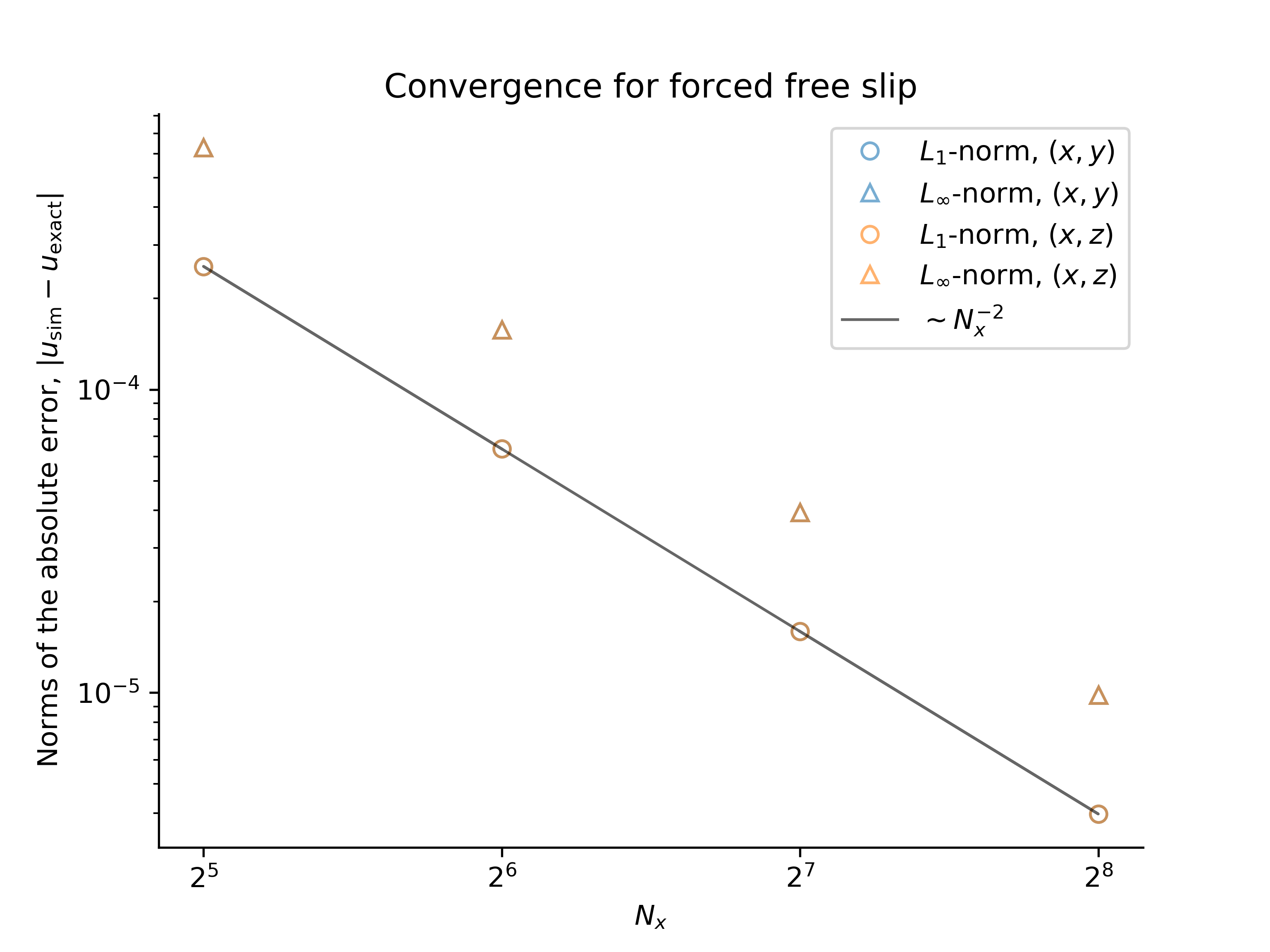
Forced, free-slip flow

A forced flow satisfying free-slip conditions at $y = 0$ and $y = \pi$ has the streamfunction

\[ \psi(x, y, t) = - \cos [x - \xi(t)] \sin (y) \, ,\]

and thus $g(y) = \sin y$. The velocity field $(u, v)$ is

\[ u = \cos (x - \xi) \cos y \, , \quad \text{and} \quad v = \sin (x - \xi) \sin y \, ,\]

which satisfies the boundary conditions $u_y |_{y=0} = u_y |_{y=\pi} = 0$ and $v |_{y=0} = v |_{y=\pi} = 0$. The vorticity forcing is

\[ F_{\omega} = - 2 \xi^\prime f_x \sin y + 4 f \sin y \, ,\]

which implies that

\[ F_v = - 2 \xi^\prime f_x \cos y + 4 f \cos y \, ,\]

and $F_v = \tfrac{1}{2} \sin 2 y$.

Forced, fixed-slip flow

A forced flow satisfying "fixed-slip" boundary conditions at $y=0$ and $y=1$ has the streamfunction

\[ \psi(x, y, t) = - \cos [x - \xi(t)] (y^3 - y^2) \, ,\]

and thus $g(y) = y^3 - y^2$. The velocity field $(u, v)$ is

\[ u = f (3y^2 - 2 y) \, , \quad \text{and} \quad v = - f_x (y^3 - y^2) \, ,\]

which satisfies the boundary conditions

\[ u |_{y=0} = 0 \, , \quad u |_{y=1} = f \, , \quad \text{and} \quad v |_{y=0} = v |_{y=1} = 0 \, .\]

The vorticity forcing is

\[ F_{\omega} = - \xi^\prime f_x (y^3 - y^2 - 6y + 2) - f f_x (12 y^3 - 12 y^2 + 4 y) + f (y^3 - y^2 - 12 y + 4) \, ,\]

which implies that

\[ F_v = \xi^\prime f_x (\tfrac{1}{4} y^4 - \tfrac{1}{3} y^3 - 3 y^2 + 2y) + f f_x (3 y^4 - 4 y^3 + 2y^2 ) - f (\tfrac{1}{4} y^4 - \tfrac{1}{3} y^3 - 6 y^2 + 4 y) \, ,\]

and

\[ F_v = 3 y^5 - 5 y^4 + 2y^3 \, .\]

We set up the problem in the same manner as the forced, free-slip problem above. Note that we also must the no-slip boundary condition $u |_{y=0} = 0$ and the time-dependent fixed-slip condition $u |_{y=1} = f$. As for the free-slip problem, we find that the error between the numerical and analytical solutions decreases with $1 / N_x^2 \sim \Delta x^2$, where $N_x$ is the number of grid points and $\Delta x$ is the spatial resolution:

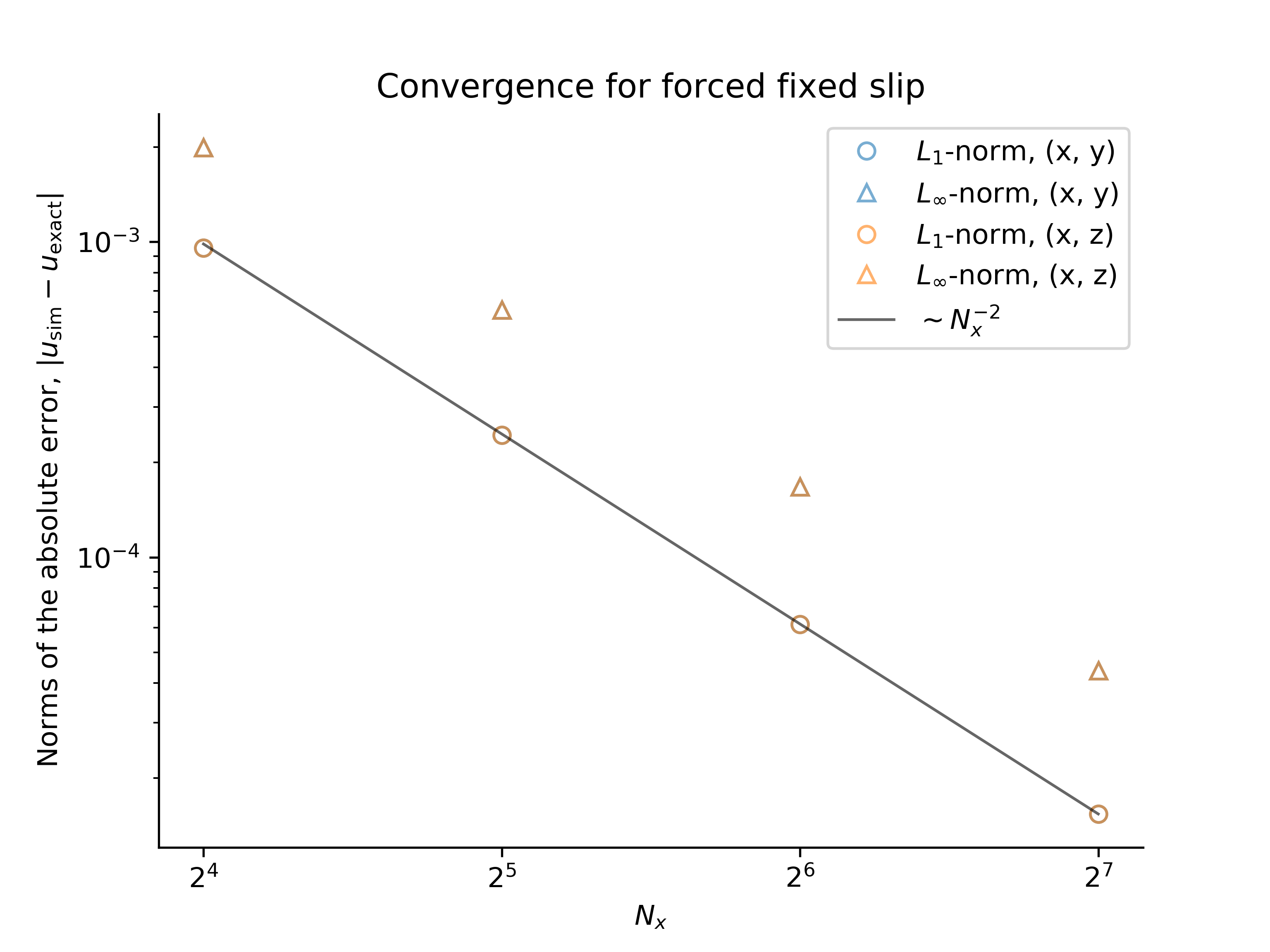
The convergence tests are performed using both $y$ and $z$ as the bounded direction.