Finite volume single stack tutorial based on the 3D Burgers + tracer equations

This tutorial implements the Burgers equations with a tracer field in a single element stack. The flow is initialized with a horizontally uniform profile of horizontal velocity and uniform initial temperature. The fluid is heated from the bottom surface. Gaussian noise is imposed to the horizontal velocity field at each node at the start of the simulation. The tutorial demonstrates how to

• Initialize a BalanceLaw in a single stack configuration;
• Return the horizontal velocity field to a given profile (e.g., large-scale advection);
• Remove any horizontal inhomogeneities or noise from the flow.

The second and third bullet points are demonstrated imposing Rayleigh friction, horizontal diffusion and 2D divergence damping to the horizontal momentum prognostic equation.

Equations solved in balance law form:

\[\begin{align} \frac{∂ ρ}{∂ t} =& - ∇ ⋅ (ρ\mathbf{u}) \\ \frac{∂ ρ\mathbf{u}}{∂ t} =& - ∇ ⋅ (-μ ∇\mathbf{u}) - ∇ ⋅ (ρ\mathbf{u} \mathbf{u}') - γ[ (ρ\mathbf{u}-ρ̄\mathbf{ū}) - (ρ\mathbf{u}-ρ̄\mathbf{ū})⋅ẑ ẑ] - ν_d ∇_h (∇_h ⋅ ρ\mathbf{u}) \\ \frac{∂ ρcT}{∂ t} =& - ∇ ⋅ (-α ∇ρcT) - ∇ ⋅ (\mathbf{u} ρcT) \end{align}\]

Boundary conditions:

\[\begin{align} z_{\mathrm{min}}: & ρ = 1 \\ z_{\mathrm{min}}: & ρ\mathbf{u} = \mathbf{0} \\ z_{\mathrm{min}}: & ρcT = ρc T_{\mathrm{fixed}} \\ z_{\mathrm{max}}: & ρ = 1 \\ z_{\mathrm{max}}: & ρ\mathbf{u} = \mathbf{0} \\ z_{\mathrm{max}}: & -α∇ρcT = 0 \end{align}\]

where

• $t$ is time
• $ρ$ is the density
• $\mathbf{u}$ is the velocity (vector)
• $\mathbf{ū}$ is the horizontally averaged velocity (vector)
• $μ$ is the dynamic viscosity tensor
• $γ$ is the Rayleigh friction frequency
• $ν_d$ is the horizontal divergence damping coefficient
• $T$ is the temperature
• $α$ is the thermal diffusivity tensor
• $c$ is the heat capacity
• $ρcT$ is the thermal energy

Solving these equations is broken down into the following steps:

1. Preliminary configuration
2. PDEs
3. Space discretization
4. Time discretization
5. Solver hooks / callbacks
6. Solve
7. Post-processing

Preliminary configuration

Loading code

First, we'll load our pre-requisites

• load external packages:

using MPI
using Distributions
using OrderedCollections
using Plots
using StaticArrays
using LinearAlgebra: Diagonal, tr

• load CLIMAParameters and set up to use it:

using CLIMAParameters
using CLIMAParameters.Planet: grav
struct EarthParameterSet <: AbstractEarthParameterSet end
const param_set = EarthParameterSet()

Main.##346.EarthParameterSet()

• load necessary ClimateMachine modules:

using ClimateMachine
using ClimateMachine.Mesh.Topologies
using ClimateMachine.Mesh.Grids
using ClimateMachine.Writers
using ClimateMachine.DGMethods
using ClimateMachine.DGMethods.NumericalFluxes
using ClimateMachine.BalanceLaws:
    BalanceLaw, Prognostic, Auxiliary, Gradient, GradientFlux, parameter_set

using ClimateMachine.Mesh.Geometry: LocalGeometry
using ClimateMachine.MPIStateArrays
using ClimateMachine.GenericCallbacks
using ClimateMachine.ODESolvers
using ClimateMachine.VariableTemplates
using ClimateMachine.SingleStackUtils
import ClimateMachine.DGMethods.FVReconstructions: FVLinear

• import necessary ClimateMachine modules: (importing enables us to

provide implementations of these structs/methods)

using ClimateMachine.Orientations:
    Orientation,
    NoOrientation,
    FlatOrientation,
    init_aux!,
    vertical_unit_vector,
    projection_tangential

import ClimateMachine.BalanceLaws:
    vars_state,
    source!,
    flux_second_order!,
    flux_first_order!,
    compute_gradient_argument!,
    compute_gradient_flux!,
    init_state_auxiliary!,
    init_state_prognostic!,
    construct_face_auxiliary_state!,
    BoundaryCondition,
    boundary_conditions,
    boundary_state!

Initialization

Define the float type (Float64 or Float32)

const FT = Float64;

Initialize ClimateMachine for CPU.

ClimateMachine.init(; disable_gpu = true);

const clima_dir = dirname(dirname(pathof(ClimateMachine)));

[1638959905.813925] [hpc-92-37:26676:0]       ib_verbs.h:84   UCX  ERROR ibv_exp_query_device(mlx5_0) returned 38: No space left on device

Load some helper functions for plotting

include(joinpath(clima_dir, "docs", "plothelpers.jl"));

Define the set of Partial Differential Equations (PDEs)

Define the model

Model parameters can be stored in the particular BalanceLaw, in this case, the BurgersEquation:

Base.@kwdef struct BurgersEquation{FT, APS, O} <: BalanceLaw
    "Parameters"
    param_set::APS
    "Orientation model"
    orientation::O
    "Heat capacity"
    c::FT = 1
    "Vertical dynamic viscosity"
    μv::FT = 1e-4
    "Horizontal dynamic viscosity"
    μh::FT = 1
    "Vertical thermal diffusivity"
    αv::FT = 1e-2
    "Horizontal thermal diffusivity"
    αh::FT = 1
    "IC Gaussian noise standard deviation"
    σ::FT = 5e-2
    "Rayleigh damping"
    γ::FT = 5
    "Domain height"
    zmax::FT = 1
    "Initial conditions for temperature"
    initialT::FT = 295.15
    "Bottom boundary value for temperature (Dirichlet boundary conditions)"
    T_bottom::FT = 300.0
    "Top flux (α∇ρcT) at top boundary (Neumann boundary conditions)"
    flux_top::FT = 0.0
    "Divergence damping coefficient (horizontal)"
    νd::FT = 1
end

Create an instance of the BurgersEquation:

orientation = FlatOrientation()

m = BurgersEquation{FT, typeof(param_set), typeof(orientation)}(
    param_set = param_set,
    orientation = orientation,
);

This model dictates the flow control, using Dynamic Multiple Dispatch, for which kernels are executed.

Define the variables

All of the methods defined in this section were imported in Loading code to let us provide implementations for our BurgersEquation as they will be used by the solver.

Specify auxiliary variables for BurgersEquation

function vars_state(m::BurgersEquation, st::Auxiliary, FT)
    @vars begin
        coord::SVector{3, FT}
        orientation::vars_state(m.orientation, st, FT)
    end
end

vars_state (generic function with 152 methods)

Specify prognostic variables, the variables solved for in the PDEs, for BurgersEquation

vars_state(::BurgersEquation, ::Prognostic, FT) =
    @vars(ρ::FT, ρu::SVector{3, FT}, ρcT::FT);

Specify state variables whose gradients are needed for BurgersEquation

vars_state(::BurgersEquation, ::Gradient, FT) =
    @vars(u::SVector{3, FT}, ρcT::FT, ρu::SVector{3, FT});

Specify gradient variables for BurgersEquation

vars_state(::BurgersEquation, ::GradientFlux, FT) = @vars(
    μ∇u::SMatrix{3, 3, FT, 9},
    α∇ρcT::SVector{3, FT},
    νd∇D::SMatrix{3, 3, FT, 9}
);

Define the compute kernels

Specify the initial values in aux::Vars, which are available in init_state_prognostic!. Note that

• this method is only called at t=0.
• aux.coord is available here because we've specified coord in vars_state(m, aux, FT).

function nodal_init_state_auxiliary!(
    m::BurgersEquation,
    aux::Vars,
    tmp::Vars,
    geom::LocalGeometry,
)
    aux.coord = geom.coord
end;

init_aux! initializes the auxiliary gravitational potential field needed for vertical projections

function init_state_auxiliary!(
    m::BurgersEquation,
    state_auxiliary::MPIStateArray,
    grid,
    direction,
)
    init_aux!(m, m.orientation, state_auxiliary, grid, direction)

    init_state_auxiliary!(
        m,
        nodal_init_state_auxiliary!,
        state_auxiliary,
        grid,
        direction,
    )
end;

Specify the initial values in state::Vars. Note that

• this method is only called at t=0.
• state.ρ, state.ρu andstate.ρcT are available here because we've specified ρ, ρu and ρcT in vars_state(m, state, FT).

function init_state_prognostic!(
    m::BurgersEquation,
    state::Vars,
    aux::Vars,
    localgeo,
    t::Real,
)
    z = aux.coord[3]
    ε1 = rand(Normal(0, m.σ))
    ε2 = rand(Normal(0, m.σ))
    state.ρ = 1
    ρu = 1 - 4 * (z - m.zmax / 2)^2 + ε1
    ρv = 1 - 4 * (z - m.zmax / 2)^2 + ε2
    ρw = 0
    state.ρu = SVector(ρu, ρv, ρw)

    state.ρcT = state.ρ * m.c * m.initialT
end;

function construct_face_auxiliary_state!(
    bl::BurgersEquation,
    aux_face::AbstractArray,
    aux_cell::AbstractArray,
    Δz::FT,
) where {FT <: Real}
    param_set = parameter_set(bl)
    _grav = FT(grav(param_set))
    var_aux = Vars{vars_state(bl, Auxiliary(), FT)}
    aux_face .= aux_cell

    if !(bl.orientation isa NoOrientation)
        var_aux(aux_face).orientation.Φ =
            var_aux(aux_cell).orientation.Φ + _grav * Δz / 2
    end
end

construct_face_auxiliary_state! (generic function with 3 methods)

The remaining methods, defined in this section, are called at every time-step in the solver by the BalanceLaw framework.

Since we have second-order fluxes, we must tell ClimateMachine to compute the gradient of ρcT, u and ρu. Here, we specify how ρcT, u and ρu are computed. Note that e.g. transform.ρcT is available here because we've specified ρcT in vars_state(m, ::Gradient, FT).

function compute_gradient_argument!(
    m::BurgersEquation,
    transform::Vars,
    state::Vars,
    aux::Vars,
    t::Real,
)
    transform.ρcT = state.ρcT
    transform.u = state.ρu / state.ρ
    transform.ρu = state.ρu
end;

Specify where in diffusive::Vars to store the computed gradient from compute_gradient_argument!. Note that:

• diffusive.μ∇u is available here because we've specified μ∇u in vars_state(m, ::GradientFlux, FT).
• ∇transform.u is available here because we've specified u in vars_state(m, ::Gradient, FT).
• diffusive.μ∇u is built using an anisotropic diffusivity tensor.
• The divergence may be computed from the trace of tensor ∇ρu.

function compute_gradient_flux!(
    m::BurgersEquation{FT},
    diffusive::Vars,
    ∇transform::Grad,
    state::Vars,
    aux::Vars,
    t::Real,
) where {FT}
    param_set = parameter_set(m)
    ∇ρu = ∇transform.ρu
    ẑ = vertical_unit_vector(m.orientation, param_set, aux)
    divergence = tr(∇ρu) - ẑ' * ∇ρu * ẑ
    diffusive.α∇ρcT = Diagonal(SVector(m.αh, m.αh, m.αv)) * ∇transform.ρcT
    diffusive.μ∇u = Diagonal(SVector(m.μh, m.μh, m.μv)) * ∇transform.u
    diffusive.νd∇D =
        Diagonal(SVector(m.νd, m.νd, FT(0))) *
        Diagonal(SVector(divergence, divergence, FT(0)))
end;

Introduce Rayleigh friction towards a target profile as a source. Note that:

• Rayleigh damping is only applied in the horizontal using the projection_tangential method.

function source!(
    m::BurgersEquation{FT},
    source::Vars,
    state::Vars,
    diffusive::Vars,
    aux::Vars,
    args...,
) where {FT}
    param_set = parameter_set(m)
    ẑ = vertical_unit_vector(m.orientation, param_set, aux)
    z = aux.coord[3]
    ρ̄ū =
        state.ρ * SVector{3, FT}(
            0.5 - 2 * (z - m.zmax / 2)^2,
            0.5 - 2 * (z - m.zmax / 2)^2,
            0.0,
        )
    ρu_p = state.ρu - ρ̄ū
    source.ρu -=
        m.γ * projection_tangential(m.orientation, param_set, aux, ρu_p)
end;

Compute advective flux. Note that:

• state.ρu is available here because we've specified ρu in vars_state(m, state, FT).

function flux_first_order!(
    m::BurgersEquation,
    flux::Grad,
    state::Vars,
    aux::Vars,
    t::Real,
    _...,
)
    flux.ρ = state.ρu

    u = state.ρu / state.ρ
    flux.ρu = state.ρu * u'
    flux.ρcT = u * state.ρcT
end;

Compute diffusive flux (e.g. $F(μ, \mathbf{u}, t) = -μ∇\mathbf{u}$ in the original PDE). Note that:

• diffusive.μ∇u is available here because we've specified μ∇u in vars_state(m, ::GradientFlux, FT).
• The divergence gradient can be written as a diffusive flux using a divergence diagonal tensor.

function flux_second_order!(
    m::BurgersEquation,
    flux::Grad,
    state::Vars,
    diffusive::Vars,
    hyperdiffusive::Vars,
    aux::Vars,
    t::Real,
)
    flux.ρcT -= diffusive.α∇ρcT
    flux.ρu -= diffusive.μ∇u
    flux.ρu -= diffusive.νd∇D
end;

Boundary conditions

Second-order terms in our equations, $∇⋅(G)$ where $G = μ∇\mathbf{u}$, are internally reformulated to first-order unknowns. Boundary conditions must be specified for all unknowns, both first-order and second-order unknowns which have been reformulated.

struct TopBC <: BoundaryCondition end;
struct BottomBC <: BoundaryCondition end;
boundary_conditions(::BurgersEquation) = (BottomBC(), TopBC());

The boundary conditions for ρ, ρu and ρcT (first order unknowns)

function boundary_state!(
    nf,
    bc::BottomBC,
    m::BurgersEquation,
    state⁺::Vars,
    aux⁺::Vars,
    n⁻,
    _...,
)
    state⁺.ρ = 1
    state⁺.ρu = SVector(0, 0, 0)
    state⁺.ρcT = state⁺.ρ * m.c * m.T_bottom
end;
function boundary_state!(
    nf,
    bc::TopBC,
    m::BurgersEquation,
    state⁺::Vars,
    aux⁺::Vars,
    n⁻,
    _...,
)
    state⁺.ρ = 1
    state⁺.ρu = SVector(0, 0, 0)
end;

The boundary conditions for ρ, ρu and ρcT are specified here for second-order unknowns

function boundary_state!(
    nf,
    bc::BottomBC,
    m::BurgersEquation,
    state⁺::Vars,
    diff⁺::Vars,
    hyperdiff⁺::Vars,
    aux⁺::Vars,
    n⁻,
    _...,
)
    state⁺.ρ = 1
    state⁺.ρu = SVector(0, 0, 0)
    state⁺.ρcT = state⁺.ρ * m.c * m.T_bottom
end;
function boundary_state!(
    nf,
    bc::TopBC,
    m::BurgersEquation,
    state⁺::Vars,
    diff⁺::Vars,
    hyperdiff⁺::Vars,
    aux⁺::Vars,
    n⁻,
    _...,
)
    state⁺.ρ = 1
    state⁺.ρu = SVector(0, 0, 0)
    diff⁺.α∇ρcT = -n⁻ * m.flux_top
end;

Spatial discretization

Prescribe polynomial order of basis functions in finite elements The second index 0 indicates that finite volume method is applied in the vertical direction

N_poly = (1, 0);

Specify the number of vertical elements

nelem_vert = 50;

Specify the domain height

zmax = m.zmax;

Establish a ClimateMachine single stack configuration

driver_config = ClimateMachine.SingleStackConfiguration(
    "BurgersEquation",
    N_poly,
    nelem_vert,
    zmax,
    param_set,
    m,
    numerical_flux_first_order = CentralNumericalFluxFirstOrder(),
    fv_reconstruction = FVLinear(),
);

ClimateMachine.array_type() = Array
┌ Info: Model composition
│     param_set = Main.##346.EarthParameterSet()
│     orientation = ClimateMachine.Orientations.FlatOrientation()
│     c = 1.0
│     μv = 0.0001
│     μh = 1.0
│     αv = 0.01
│     αh = 1.0
│     σ = 0.05
│     γ = 5.0
│     zmax = 1.0
│     initialT = 295.15
│     T_bottom = 300.0
│     flux_top = 0.0
│     νd = 1.0
└ @ ClimateMachine /central/scratch/climaci/climatemachine-docs/1430/climatemachine-docs/src/Driver/driver_configs.jl:188
┌ Info: Defining `prognostic_vars` and
│ `eq_tends` for BurgersEquation will
│ enable printing a table of tendencies.
└ @ ClimateMachine.BalanceLaws /central/scratch/climaci/climatemachine-docs/1430/climatemachine-docs/src/BalanceLaws/show_tendencies.jl:65
┌ Info: Establishing single stack configuration for BurgersEquation
│     precision               = Float64
│     horiz polynomial order  = 1
│     vert polynomial order   = 0
│     domain_min              = 0.00 m, 0.00 m, 0.00 m
│     domain_max              = 1.00 m, 1.00 m, 1.00 m
│     # vert elems            = 50
│     MPI ranks               = 1
│     min(Δ_horz)             = 1.00 m
│     min(Δ_vert)             = 0.02 m
└ @ ClimateMachine /central/scratch/climaci/climatemachine-docs/1430/climatemachine-docs/src/Driver/driver_configs.jl:612

Time discretization

Specify simulation time (SI units)

t0 = FT(0);
timeend = FT(1);

We'll define the time-step based on the Fourier number and the Courant number of the flow

Δ = min_node_distance(driver_config.grid)

given_Fourier = FT(0.5);
Fourier_bound = given_Fourier * Δ^2 / max(m.αh, m.μh, m.νd);
Courant_bound = FT(0.5) * Δ;
dt = min(Fourier_bound, Courant_bound)

0.00019999999999999814

Configure a ClimateMachine solver.

This initializes the state vector and allocates memory for the solution in space (dg has the model m, which describes the PDEs as well as the function used for initialization). This additionally initializes the ODE solver, by default an explicit Low-Storage Runge-Kutta method.

solver_config =
    ClimateMachine.SolverConfiguration(t0, timeend, driver_config, ode_dt = dt);

┌ Info: Initializing BurgersEquation
└ @ ClimateMachine /central/scratch/climaci/climatemachine-docs/1430/climatemachine-docs/src/Driver/solver_configs.jl:185

Inspect the initial conditions for a single nodal stack

Let's export plots of the initial state

output_dir = @__DIR__;

mkpath(output_dir);

z_scale = 100 # convert from meters to cm
z_key = "z"
z_label = "z [cm]"
z = get_z(driver_config.grid; z_scale = z_scale)
state_vars = get_vars_from_nodal_stack(
    driver_config.grid,
    solver_config.Q,
    vars_state(m, Prognostic(), FT),
);

Create an array to store the solution:

state_data = Dict[state_vars]  # store initial condition at ``t=0``
time_data = FT[0]                                      # store time data

1-element Array{Float64,1}:
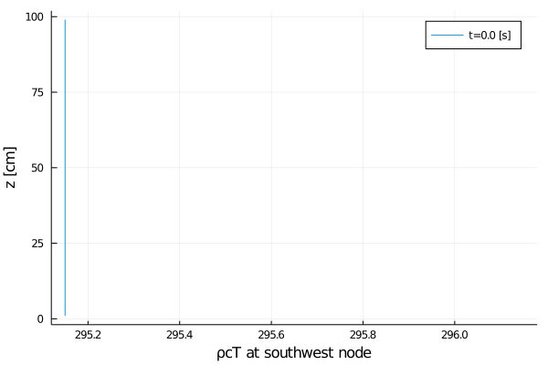
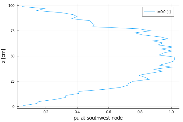
 0.0

Generate plots of initial conditions for the southwest nodal stack

export_plot(
    z,
    time_data,
    state_data,
    ("ρcT",),
    joinpath(output_dir, "initial_condition_T_nodal_fvm.png");
    xlabel = "ρcT at southwest node",
    ylabel = z_label,
);
export_plot(
    z,
    time_data,
    state_data,
    ("ρu[1]",),
    joinpath(output_dir, "initial_condition_u_nodal_fvm.png");
    xlabel = "ρu at southwest node",
    ylabel = z_label,
);
export_plot(
    z,
    time_data,
    state_data,
    ("ρu[2]",),
    joinpath(output_dir, "initial_condition_v_nodal_fvm.png");
    xlabel = "ρv at southwest node",
    ylabel = z_label,
);

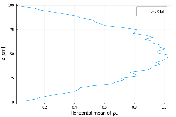
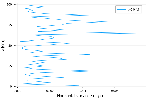
Inspect the initial conditions for the horizontal averages

Horizontal statistics of variables

state_vars_var = get_horizontal_variance(
    driver_config.grid,
    solver_config.Q,
    vars_state(m, Prognostic(), FT),
);

state_vars_avg = get_horizontal_mean(
    driver_config.grid,
    solver_config.Q,
    vars_state(m, Prognostic(), FT),
);

data_avg = Dict[state_vars_avg]
data_var = Dict[state_vars_var]

export_plot(
    z,
    time_data,
    data_avg,
    ("ρu[1]",),
    joinpath(output_dir, "initial_condition_avg_u_fvm.png");
    xlabel = "Horizontal mean of ρu",
    ylabel = z_label,
);
export_plot(
    z,
    time_data,
    data_var,
    ("ρu[1]",),
    joinpath(output_dir, "initial_condition_variance_u_fvm.png");
    xlabel = "Horizontal variance of ρu",
    ylabel = z_label,
);

Solver hooks / callbacks

Define the number of outputs from t0 to timeend

const n_outputs = 5;
const every_x_simulation_time = timeend / n_outputs;

Create a dictionary for z coordinate (and convert to cm) NCDatasets IO:

dims = OrderedDict(z_key => collect(z));

Create dictionaries to store outputs:

data_var = Dict[Dict([k => Dict() for k in 0:n_outputs]...),]
data_var[1] = state_vars_var

data_avg = Dict[Dict([k => Dict() for k in 0:n_outputs]...),]
data_avg[1] = state_vars_avg

data_nodal = Dict[Dict([k => Dict() for k in 0:n_outputs]...),]
data_nodal[1] = state_vars

OrderedCollections.OrderedDict{Any,Any} with 5 entries:
  "ρ" => [1.0, 1.0, 1.0, 1.0, 1.0, 1.0, 1.0, 1.0, 1.0, 1.0, 1.0, 1.0, 1.0, 1.0, 1.0, 1.0, 1.0, 1.0, 1.0, 1.0, 1.0, 1.0, 1.0, 1.0, 1.0, 1.0, 1.0, 1.0, 1.0, 1.0, 1.0, 1.0, 1.0, 1.0, 1.0, 1.0, 1.0, 1.0, 1.0, 1.0, 1.0, 1.0, 1.0, 1.0, 1.0, 1.0, 1.0, 1.0, 1.0, 1.0]
  "ρu[1]" => [0.0544644, 0.142898, 0.155317, 0.257231, 0.324262, 0.327148, 0.409897, 0.409635, 0.571115, 0.674334, 0.720991, 0.726357, 0.75781, 0.859654, 0.830187, 0.793305, 0.863497, 0.942916, 0.887076, 1.00169, 0.921864, 0.976861, 1.01394, 1.02173, 1.01779, 0.920194, 0.947816, 1.00464, 0.93448, 1.0113, 0.914583, 0.945433, 0.881627, 0.98008, 0.928994, 0.813707, 0.766689, 0.869026, 0.792281, 0.498607, 0.508231, 0.491064, 0.481125, 0.363651, 0.399169, 0.374607, 0.296449, 0.142297, 0.192953, 0.0461905]
  "ρu[2]" => [0.0587198, 0.137971, 0.101308, 0.327247, 0.388723, 0.374836, 0.50887, 0.481557, 0.533594, 0.549251, 0.638346, 0.724401, 0.709284, 0.768469, 0.887967, 0.789017, 0.812834, 0.887552, 0.883889, 0.916358, 0.959847, 1.04289, 1.02026, 1.03999, 1.03337, 1.01447, 0.905507, 1.02339, 1.00865, 0.924855, 1.00836, 0.801372, 0.864039, 0.803445, 0.921392, 0.840046, 0.800594, 0.85948, 0.636908, 0.602009, 0.531437, 0.620397, 0.572658, 0.419077, 0.39049, 0.324175, 0.303623, 0.0638146, 0.0902433, 0.0902286]
  "ρu[3]" => [0.0, 0.0, 0.0, 0.0, 0.0, 0.0, 0.0, 0.0, 0.0, 0.0, 0.0, 0.0, 0.0, 0.0, 0.0, 0.0, 0.0, 0.0, 0.0, 0.0, 0.0, 0.0, 0.0, 0.0, 0.0, 0.0, 0.0, 0.0, 0.0, 0.0, 0.0, 0.0, 0.0, 0.0, 0.0, 0.0, 0.0, 0.0, 0.0, 0.0, 0.0, 0.0, 0.0, 0.0, 0.0, 0.0, 0.0, 0.0, 0.0, 0.0]
  "ρcT" => [295.15, 295.15, 295.15, 295.15, 295.15, 295.15, 295.15, 295.15, 295.15, 295.15, 295.15, 295.15, 295.15, 295.15, 295.15, 295.15, 295.15, 295.15, 295.15, 295.15, 295.15, 295.15, 295.15, 295.15, 295.15, 295.15, 295.15, 295.15, 295.15, 295.15, 295.15, 295.15, 295.15, 295.15, 295.15, 295.15, 295.15, 295.15, 295.15, 295.15, 295.15, 295.15, 295.15, 295.15, 295.15, 295.15, 295.15, 295.15, 295.15, 295.15]

The ClimateMachine's time-steppers provide hooks, or callbacks, which allow users to inject code to be executed at specified intervals. In this callback, the state variables are collected, combined into a single OrderedDict and written to a NetCDF file (for each output step).

callback = GenericCallbacks.EveryXSimulationTime(every_x_simulation_time) do
    state_vars_var = get_horizontal_variance(
        driver_config.grid,
        solver_config.Q,
        vars_state(m, Prognostic(), FT),
    )
    state_vars_avg = get_horizontal_mean(
        driver_config.grid,
        solver_config.Q,
        vars_state(m, Prognostic(), FT),
    )
    state_vars = get_vars_from_nodal_stack(
        driver_config.grid,
        solver_config.Q,
        vars_state(m, Prognostic(), FT),
        i = 1,
        j = 1,
    )
    push!(data_var, state_vars_var)
    push!(data_avg, state_vars_avg)
    push!(data_nodal, state_vars)
    push!(time_data, gettime(solver_config.solver))
    nothing
end;

Solve

This is the main ClimateMachine solver invocation. While users do not have access to the time-stepping loop, code may be injected via user_callbacks, which is a Tuple of GenericCallbacks.

ClimateMachine.invoke!(solver_config; user_callbacks = (callback,))

1.0018379905465364

Post-processing

Our solution has now been calculated and exported to NetCDF files in output_dir.

Let's plot the horizontal statistics of ρu and ρcT, as well as the evolution of ρu for the southwest nodal stack:

export_plot(
    z,
    time_data,
    data_avg,
    ("ρu[1]"),
    joinpath(output_dir, "solution_vs_time_u_avg_fvm.png");
    xlabel = "Horizontal mean of ρu",
    ylabel = z_label,
);
export_plot(
    z,
    time_data,
    data_var,
    ("ρu[1]"),
    joinpath(output_dir, "variance_vs_time_u_fvm.png");
    xlabel = "Horizontal variance of ρu",
    ylabel = z_label,
);
export_plot(
    z,
    time_data,
    data_avg,
    ("ρcT"),
    joinpath(output_dir, "solution_vs_time_T_avg_fvm.png");
    xlabel = "Horizontal mean of ρcT",
    ylabel = z_label,
);
export_plot(
    z,
    time_data,
    data_var,
    ("ρcT"),
    joinpath(output_dir, "variance_vs_time_T_fvm.png");
    xlabel = "Horizontal variance of ρcT",
    ylabel = z_label,
);
export_plot(
    z,
    time_data,
    data_nodal,
    ("ρu[1]"),
    joinpath(output_dir, "solution_vs_time_u_nodal_fvm.png");
    xlabel = "ρu at southwest node",
    ylabel = z_label,
);

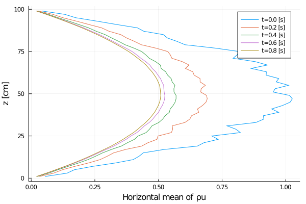
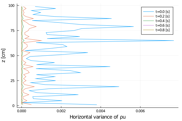
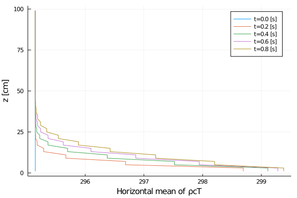
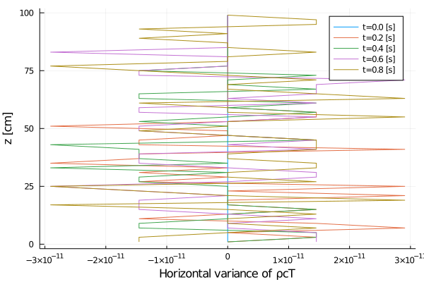
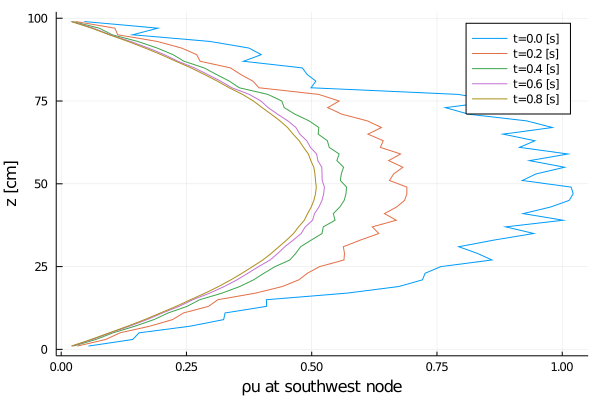
Rayleigh friction returns the horizontal velocity to the objective profile on the timescale of the simulation (1 second), since γ∼1. The horizontal viscosity and 2D divergence damping act to reduce the horizontal variance over the same timescale. The initial Gaussian noise is propagated to the temperature field through advection. The horizontal diffusivity acts to reduce this ρcT variance in time, although in a longer timescale.

To run this file, and inspect the solution, include this tutorial in the Julia REPL with:

include(joinpath("tutorials", "Atmos", "burgers_single_stack.jl"))

This page was generated using Literate.jl.