Solving the heat equation in soil

This tutorial shows how to use CliMA code to solve the heat equation in soil. For background on the heat equation in general, and how to solve it using CliMA code, please see the heat_equation.jl tutorial.

The version of the heat equation we are solving here assumes no sources or sinks and no flow of liquid water. It takes the form

$\frac{∂ ρe_{int}}{∂ t} = ∇ ⋅ κ(θ_l, θ_i; ν, ...) ∇T$

Here

$t$ is the time (s),

$z$ is the location in the vertical (m),

$ρe_{int}$ is the volumetric internal energy of the soil (J/m^3),

$T$ is the temperature of the soil (K),

$κ$ is the thermal conductivity (W/m/K),

$ϑ_l$ is the augmented volumetric liquid water fraction,

$θ_i$ is the volumetric ice fraction, and

$ν, ...$ denotes parameters relating to soil type, such as porosity.

We will solve this equation in an effectively 1-d domain with $z ∈ [-1,0]$, and with the following boundary and initial conditions:

$T(t=0, z) = 277.15^\circ K$

$T(t, z = 0) = 288.15^\circ K$

$-κ ∇T(t, z = -1) = 0 ẑ$

The temperature $T$ and volumetric internal energy $ρe_{int}$ are related as

$ρe_{int} = ρc_s (θ_l, θ_i; ν, ...) (T - T_0) - θ_i ρ_i LH_{f0}$

where

$ρc_s$ is the volumetric heat capacity of the soil (J/m^3/K),

$T_0$ is the freezing temperature of water,

$ρ_i$ is the density of ice (kg/m^3), and

$LH_{f0}$ is the latent heat of fusion at $T_0$.

In this tutorial, we will use a PrescribedWaterModel. This option allows the user to specify a function for the spatial and temporal behavior of θ_i and θ_l; it does not solve Richard's equation for the evolution of moisture. Please see the tutorials in the Soil/Coupled/ folder or the Soil/Water/ folder for information on solving Richard's equation, either coupled or uncoupled from the heat equation, respectively.

Import necessary modules

External (non - CliMA) modules

using MPI
using OrderedCollections
using StaticArrays
using Statistics
using Dierckx
using Plots
using DelimitedFiles

CliMA Parameters

using CLIMAParameters
using CLIMAParameters.Planet: ρ_cloud_liq, ρ_cloud_ice, cp_l, cp_i, T_0, LH_f0

ClimateMachine modules

using ClimateMachine
using ClimateMachine.Land
using ClimateMachine.Land.SoilWaterParameterizations
using ClimateMachine.Land.SoilHeatParameterizations
using ClimateMachine.Mesh.Topologies
using ClimateMachine.Mesh.Grids
using ClimateMachine.DGMethods
using ClimateMachine.DGMethods.NumericalFluxes
using ClimateMachine.DGMethods: BalanceLaw, LocalGeometry
using ClimateMachine.MPIStateArrays
using ClimateMachine.GenericCallbacks
using ClimateMachine.ODESolvers
using ClimateMachine.VariableTemplates
using ClimateMachine.SingleStackUtils
using ClimateMachine.BalanceLaws:
    BalanceLaw,
    Prognostic,
    Auxiliary,
    Gradient,
    GradientFlux,
    vars_state,
    parameter_set
import ClimateMachine.DGMethods: calculate_dt
using ArtifactWrappers

Preliminary set-up

Get the parameter set, which holds constants used across CliMA models.

struct EarthParameterSet <: AbstractEarthParameterSet end
const param_set = EarthParameterSet();

Initialize and pick a floating point precision.

ClimateMachine.init()
const FT = Float32;

[1638959942.347403] [hpc-92-37:26674:0]       ib_verbs.h:84   UCX  ERROR ibv_exp_query_device(mlx5_0) returned 38: No space left on device

Load functions that will help with plotting

const clima_dir = dirname(dirname(pathof(ClimateMachine)));
include(joinpath(clima_dir, "docs", "plothelpers.jl"));

Determine soil parameters

Below are the soil component fractions for various soil texture classes, from B.J. Cosby al. (1984) and G. Bonan (2019). Note that these fractions are volumetric fractions, relative to other soil solids, i.e. not including pore space. These are denoted ν_ss_i; the CliMA Land Documentation uses the symbol ν_i to denote the volumetric fraction of a soil component i relative to the soil, including pore space.

ν_ss_silt_array =
    FT.(
        [5.0, 12.0, 32.0, 70.0, 39.0, 15.0, 56.0, 34.0, 6.0, 47.0, 20.0] ./
        100.0,
    )
ν_ss_quartz_array =
    FT.(
        [92.0, 82.0, 58.0, 17.0, 43.0, 58.0, 10.0, 32.0, 52.0, 6.0, 22.0] ./
        100.0,
    )
ν_ss_clay_array =
    FT.(
        [3.0, 6.0, 10.0, 13.0, 18.0, 27.0, 34.0, 34.0, 42.0, 47.0, 58.0] ./
        100.0,
    )
porosity_array =
    FT.([
        0.395,
        0.410,
        0.435,
        0.485,
        0.451,
        0.420,
        0.477,
        0.476,
        0.426,
        0.492,
        0.482,
    ]);

The soil types that correspond to array elements above are, in order, sand, loamy sand, sandy loam, silty loam, loam, sandy clay loam, silty clay loam, clay loam, sandy clay, silty clay, and clay.

Here we choose the soil type to be sandy. The soil column is uniform in space and time.

soil_type_index = 1
ν_ss_minerals =
    ν_ss_clay_array[soil_type_index] + ν_ss_silt_array[soil_type_index]
ν_ss_quartz = ν_ss_quartz_array[soil_type_index]
porosity = porosity_array[soil_type_index];

This tutorial additionally compares the output of a ClimateMachine simulation with that of Supplemental Program 2, Chapter 5, of G. Bonan (2019). We found this useful as it allows us compare results from our code against a published version.

The simulation code of G. Bonan (2019) employs a formalism for the thermal conductivity κ based on O. Johanson (1977). It assumes no organic matter, and only requires the volumetric fraction of soil solids for quartz and other minerals. ClimateMachine employs the formalism of V. Balland , P. A. Arp (2005), which requires the fraction of soil solids for quartz, gravel, organic matter, and other minerals. Yongjiu Dai al. (2019) found the model of V. Balland , P. A. Arp (2005) to better match measured soil properties across a range of soil types.

To compare the output of the two simulations, we set the organic matter content and gravel content to zero in the CliMA model. The remaining soil components (quartz and other minerals) match between the two. We also run the simulation for relatively wet soil (water content at 80% of porosity). Under these conditions, the two formulations for κ, though taking different functional forms, are relatively consistent. The differences between models are important for soil with organic material and for soil that is relatively dry.

ν_ss_om = FT(0.0)
ν_ss_gravel = FT(0.0);

We next calculate a few intermediate quantities needed for the determination of the thermal conductivity (V. Balland , P. A. Arp (2005)). These include the conductivity of the solid material, the conductivity of saturated soil, and the conductivity of frozen saturated soil.

κ_quartz = FT(7.7) # W/m/K
κ_minerals = FT(2.5) # W/m/K
κ_om = FT(0.25) # W/m/K
κ_liq = FT(0.57) # W/m/K
κ_ice = FT(2.29); # W/m/K

The particle density of soil solids in moisture-free soil is taken as a constant, across soil types, as in G. Bonan (2019). This is a good estimate for organic material free soil. The user is referred to V. Balland , P. A. Arp (2005) for a more general expression.

ρp = FT(2700) # kg/m^3
κ_solid = k_solid(ν_ss_om, ν_ss_quartz, κ_quartz, κ_minerals, κ_om)
κ_sat_frozen = ksat_frozen(κ_solid, porosity, κ_ice)
κ_sat_unfrozen = ksat_unfrozen(κ_solid, porosity, κ_liq);

The thermal conductivity of dry soil is also required, but this is calculated internally using the expression of [3].

The volumetric specific heat of dry soil is chosen so as to match Bonan's simulation. The user could instead compute this using a volumetric fraction weighted average across soil components.

ρc_ds = FT((1 - porosity) * 1.926e06) # J/m^3/K

1.16523f6

Finally, we store the soil-specific parameters and functions in a place where they will be accessible to the model during integration.

soil_param_functions = SoilParamFunctions(
    FT;
    porosity = porosity,
    ν_ss_gravel = ν_ss_gravel,
    ν_ss_om = ν_ss_om,
    ν_ss_quartz = ν_ss_quartz,
    ρc_ds = ρc_ds,
    ρp = ρp,
    κ_solid = κ_solid,
    κ_sat_unfrozen = κ_sat_unfrozen,
    κ_sat_frozen = κ_sat_frozen,
);

Initial and Boundary conditions

We will be using a PrescribedWaterModel, where the user supplies the augmented liquid fraction and ice fraction as functions of space and time. Since we are not implementing phase changes, it makes sense to either have entirely liquid or frozen water. This tutorial shows liquid water.

Because the two models for thermal conductivity agree well for wetter soil, we'll choose that here. However, the user could also explore how they differ by choosing drier soil.

Please note that if the user uses a mix of liquid and frozen water, that they must ensure that the total water content does not exceed porosity.

prescribed_augmented_liquid_fraction = FT(porosity * 0.8)
prescribed_volumetric_ice_fraction = FT(0.0);

Choose boundary and initial conditions for heat that will not lead to freezing of water:

heat_surface_state = (aux, t) -> eltype(aux)(288.15)
heat_bottom_flux = (aux, t) -> eltype(aux)(0.0)
T_init = (aux) -> eltype(aux)(275.15);

The boundary value problem in this case, with two spatial derivatives, requires a boundary condition at the top of the domain and the bottom. Here we choose to specify a bottom flux condition, and a top state condition. Our problem is effectively 1D, so we do not need to specify lateral boundary conditions.

bc = LandDomainBC(
    bottom_bc = LandComponentBC(soil_heat = Neumann(heat_bottom_flux)),
    surface_bc = LandComponentBC(soil_heat = Dirichlet(heat_surface_state)),
);

We also need to define a function init_soil!, which initializes all of the prognostic variables (here, we only have ρe_int, the volumetric internal energy). The initialization is based on user-specified initial conditions. Note that the user provides initial conditions for heat based on the temperature - init_soil! also converts between T and ρe_int.

function init_soil!(land, state, aux, localgeo, time)
    param_set = parameter_set(land)
    ϑ_l, θ_i = get_water_content(land.soil.water, aux, state, time)
    θ_l = volumetric_liquid_fraction(ϑ_l, land.soil.param_functions.porosity)
    ρc_ds = land.soil.param_functions.ρc_ds
    ρc_s = volumetric_heat_capacity(θ_l, θ_i, ρc_ds, param_set)

    state.soil.heat.ρe_int = volumetric_internal_energy(
        θ_i,
        ρc_s,
        land.soil.heat.initialT(aux),
        param_set,
    )
end;

Create the model structure

soil_water_model = PrescribedWaterModel(
    (aux, t) -> prescribed_augmented_liquid_fraction,
    (aux, t) -> prescribed_volumetric_ice_fraction,
);

soil_heat_model = SoilHeatModel(FT; initialT = T_init);

The full soil model requires a heat model and a water model, as well as the soil parameter functions:

m_soil = SoilModel(soil_param_functions, soil_water_model, soil_heat_model);

The equations being solved in this tutorial have no sources or sinks:

sources = ();

Finally, we create the LandModel. In more complex land models, this would include the canopy, carbon state of the soil, etc.

m = LandModel(
    param_set,
    m_soil;
    boundary_conditions = bc,
    source = sources,
    init_state_prognostic = init_soil!,
);

Specify the numerical details

These include the resolution, domain boundaries, integration time, Courant number, and ODE solver.

N_poly = 1
nelem_vert = 100

zmax = FT(0)
zmin = FT(-1)

driver_config = ClimateMachine.SingleStackConfiguration(
    "LandModel",
    N_poly,
    nelem_vert,
    zmax,
    param_set,
    m;
    zmin = zmin,
    numerical_flux_first_order = CentralNumericalFluxFirstOrder(),
);

ClimateMachine.array_type() = Array
┌ Info: Model composition
│     param_set = Main.##350.EarthParameterSet()
│     soil = ClimateMachine.Land.SoilModel{ClimateMachine.Land.SoilParamFunctions{Float32,Float32,Float32,Float32,Float32,Float32,Float32,Float32,Float32,Float32,Float32,Float32,Float32,ClimateMachine.Land.WaterParamFunctions{Float32,ClimateMachine.Land.var"#4#16"{Float32,ClimateMachine.Land.var"#9#21"},ClimateMachine.Land.var"#6#18"{Float32,ClimateMachine.Land.var"#10#22"},ClimateMachine.Land.var"#8#20"{Float32,ClimateMachine.Land.var"#11#23"}}},ClimateMachine.Land.PrescribedWaterModel{Main.##350.var"#17#19",Main.##350.var"#18#20"},ClimateMachine.Land.SoilHeatModel{Float32,Main.##350.var"#15#16"}}(ClimateMachine.Land.SoilParamFunctions{Float32,Float32,Float32,Float32,Float32,Float32,Float32,Float32,Float32,Float32,Float32,Float32,Float32,ClimateMachine.Land.WaterParamFunctions{Float32,ClimateMachine.Land.var"#4#16"{Float32,ClimateMachine.Land.var"#9#21"},ClimateMachine.Land.var"#6#18"{Float32,ClimateMachine.Land.var"#10#22"},ClimateMachine.Land.var"#8#20"{Float32,ClimateMachine.Land.var"#11#23"}}}(0.395f0, 0.0f0, 0.0f0, 0.92f0, 1.16523f6, 2700.0f0, 7.03731f0, 2.6076639f0, 4.5166464f0, 0.24f0, 18.1f0, 0.053f0, ClimateMachine.Land.WaterParamFunctions{Float32,ClimateMachine.Land.var"#4#16"{Float32,ClimateMachine.Land.var"#9#21"},ClimateMachine.Land.var"#6#18"{Float32,ClimateMachine.Land.var"#10#22"},ClimateMachine.Land.var"#8#20"{Float32,ClimateMachine.Land.var"#11#23"}}(ClimateMachine.Land.var"#4#16"{Float32,ClimateMachine.Land.var"#9#21"}(ClimateMachine.Land.var"#9#21"()), ClimateMachine.Land.var"#6#18"{Float32,ClimateMachine.Land.var"#10#22"}(ClimateMachine.Land.var"#10#22"()), ClimateMachine.Land.var"#8#20"{Float32,ClimateMachine.Land.var"#11#23"}(ClimateMachine.Land.var"#11#23"()))), ClimateMachine.Land.PrescribedWaterModel{Main.##350.var"#17#19",Main.##350.var"#18#20"}(Main.##350.var"#17#19"(), Main.##350.var"#18#20"()), ClimateMachine.Land.SoilHeatModel{Float32,Main.##350.var"#15#16"}(Main.##350.var"#15#16"()))
│     surface = ClimateMachine.Land.SurfaceFlow.NoSurfaceFlowModel()
│     boundary_conditions = ClimateMachine.Land.LandDomainBC{ClimateMachine.Land.LandComponentBC{ClimateMachine.Land.NoBC,ClimateMachine.Land.Dirichlet{Main.##350.var"#11#12"},ClimateMachine.Land.NoBC},ClimateMachine.Land.LandComponentBC{ClimateMachine.Land.NoBC,ClimateMachine.Land.Neumann{Main.##350.var"#13#14"},ClimateMachine.Land.NoBC},ClimateMachine.Land.LandComponentBC{ClimateMachine.Land.NoBC,ClimateMachine.Land.NoBC,ClimateMachine.Land.NoBC},ClimateMachine.Land.LandComponentBC{ClimateMachine.Land.NoBC,ClimateMachine.Land.NoBC,ClimateMachine.Land.NoBC},ClimateMachine.Land.LandComponentBC{ClimateMachine.Land.NoBC,ClimateMachine.Land.NoBC,ClimateMachine.Land.NoBC},ClimateMachine.Land.LandComponentBC{ClimateMachine.Land.NoBC,ClimateMachine.Land.NoBC,ClimateMachine.Land.NoBC}}(ClimateMachine.Land.LandComponentBC{ClimateMachine.Land.NoBC,ClimateMachine.Land.Dirichlet{Main.##350.var"#11#12"},ClimateMachine.Land.NoBC}(ClimateMachine.Land.NoBC(), ClimateMachine.Land.Dirichlet{Main.##350.var"#11#12"}(Main.##350.var"#11#12"()), ClimateMachine.Land.NoBC()), ClimateMachine.Land.LandComponentBC{ClimateMachine.Land.NoBC,ClimateMachine.Land.Neumann{Main.##350.var"#13#14"},ClimateMachine.Land.NoBC}(ClimateMachine.Land.NoBC(), ClimateMachine.Land.Neumann{Main.##350.var"#13#14"}(Main.##350.var"#13#14"()), ClimateMachine.Land.NoBC()), ClimateMachine.Land.LandComponentBC{ClimateMachine.Land.NoBC,ClimateMachine.Land.NoBC,ClimateMachine.Land.NoBC}(ClimateMachine.Land.NoBC(), ClimateMachine.Land.NoBC(), ClimateMachine.Land.NoBC()), ClimateMachine.Land.LandComponentBC{ClimateMachine.Land.NoBC,ClimateMachine.Land.NoBC,ClimateMachine.Land.NoBC}(ClimateMachine.Land.NoBC(), ClimateMachine.Land.NoBC(), ClimateMachine.Land.NoBC()), ClimateMachine.Land.LandComponentBC{ClimateMachine.Land.NoBC,ClimateMachine.Land.NoBC,ClimateMachine.Land.NoBC}(ClimateMachine.Land.NoBC(), ClimateMachine.Land.NoBC(), ClimateMachine.Land.NoBC()), ClimateMachine.Land.LandComponentBC{ClimateMachine.Land.NoBC,ClimateMachine.Land.NoBC,ClimateMachine.Land.NoBC}(ClimateMachine.Land.NoBC(), ClimateMachine.Land.NoBC(), ClimateMachine.Land.NoBC()))
│     source = ()
│     source_dt = DispatchedTuples.DispatchedTuple{Tuple{},DispatchedTuples.NoDefaults} with 0 entries:
│   default => ()
│ 
│     init_state_prognostic = init_soil!
└ @ ClimateMachine /central/scratch/climaci/climatemachine-docs/1430/climatemachine-docs/src/Driver/driver_configs.jl:188
┌ Warning: This table is temporarily incomplete
└ @ ClimateMachine.BalanceLaws /central/scratch/climaci/climatemachine-docs/1430/climatemachine-docs/src/BalanceLaws/show_tendencies.jl:51

PDE: ∂_t Y_i + (∇•F_1(Y))_i + (∇•F_2(Y,G)))_i = (S(Y,G))_i
┌──────────────────────────┬──────────────────┬───────────────────┬────────┐
│                 Equation │ Flux{FirstOrder} │ Flux{SecondOrder} │ Source │
│                    (Y_i) │            (F_1) │             (F_2) │    (S) │
├──────────────────────────┼──────────────────┼───────────────────┼────────┤
│ VolumetricInternalEnergy │               () │    (DiffHeatFlux) │     () │
└──────────────────────────┴──────────────────┴───────────────────┴────────┘

┌ Info: Establishing single stack configuration for LandModel
│     precision               = Float32
│     horiz polynomial order  = 1
│     vert polynomial order   = 1
│     domain_min              = 0.00 m, 0.00 m, -1.00 m
│     domain_max              = 1.00 m, 1.00 m, 0.00 m
│     # vert elems            = 100
│     MPI ranks               = 1
│     min(Δ_horz)             = 1.00 m
│     min(Δ_vert)             = 0.01 m
└ @ ClimateMachine /central/scratch/climaci/climatemachine-docs/1430/climatemachine-docs/src/Driver/driver_configs.jl:612

In this tutorial, we determine a timestep based on a Courant number ( also called a Fourier number in the context of the heat equation). In short, we can use the parameters of the model (κ and ρc_s), along with with the size of elements of the grid used for discretizing the PDE, to estimate a natural timescale for heat transfer across a grid cell. Because we are using an explicit ODE solver, the timestep should be a fraction of this in order to resolve the dynamics.

This allows us to automate, to a certain extent, choosing a value for the timestep, even as we switch between soil types.

function calculate_dt(dg, model::LandModel, Q, Courant_number, t, direction)
    Δt = one(eltype(Q))
    CFL = DGMethods.courant(diffusive_courant, dg, model, Q, Δt, t, direction)
    return Courant_number / CFL
end

function diffusive_courant(
    m::LandModel,
    state::Vars,
    aux::Vars,
    diffusive::Vars,
    Δx,
    Δt,
    t,
    direction,
)
    param_set = parameter_set(m)
    soil = m.soil
    ϑ_l, θ_i = get_water_content(soil.water, aux, state, t)
    θ_l = volumetric_liquid_fraction(ϑ_l, soil.param_functions.porosity)
    κ_dry = k_dry(param_set, soil.param_functions)
    S_r = relative_saturation(θ_l, θ_i, soil.param_functions.porosity)
    kersten = kersten_number(θ_i, S_r, soil.param_functions)
    κ_sat = saturated_thermal_conductivity(
        θ_l,
        θ_i,
        soil.param_functions.κ_sat_unfrozen,
        soil.param_functions.κ_sat_frozen,
    )
    κ = thermal_conductivity(κ_dry, kersten, κ_sat)
    ρc_ds = soil.param_functions.ρc_ds
    ρc_s = volumetric_heat_capacity(θ_l, θ_i, ρc_ds, param_set)
    return Δt * κ / (Δx * Δx * ρc_ds)
end


t0 = FT(0)
timeend = FT(60 * 60 * 3)
Courant_number = FT(0.5) # much bigger than this leads to domain errors

solver_config = ClimateMachine.SolverConfiguration(
    t0,
    timeend,
    driver_config;
    Courant_number = Courant_number,
    CFL_direction = VerticalDirection(),
);

┌ Info: Initializing LandModel
└ @ ClimateMachine /central/scratch/climaci/climatemachine-docs/1430/climatemachine-docs/src/Driver/solver_configs.jl:185

Run the integration

ClimateMachine.invoke!(solver_config);
state_types = (Prognostic(), Auxiliary())
dons = dict_of_nodal_states(solver_config, state_types; interp = true)

OrderedCollections.OrderedDict{String,Array{Float32,1}} with 5 entries:
  "soil.heat.ρe_int" => Float32[4.94801f6, 4.94799f6, 4.948f6, 4.94801f6, 4.94798f6, 4.94798f6, 4.948f6, 4.94798f6, 4.94802f6, 4.94798f6, 4.948f6, 4.94797f6, 4.94802f6, 4.94796f6, 4.94798f6, 4.948f6, 4.948f6, 4.94798f6, 4.94799f6, 4.94799f6, 4.94799f6, 4.94801f6, 4.94798f6, 4.94802f6, 4.94796f6, 4.94799f6, 4.94798f6, 4.94799f6, 4.94799f6, 4.94799f6, 4.94798f6, 4.94801f6, 4.94803f6, 4.94809f6, 4.94816f6, 4.94823f6, 4.94832f6, 4.94842f6, 4.94864f6, 4.94889f6, 4.94919f6, 4.94963f6, 4.95021f6, 4.95094f6, 4.95191f6, 4.95317f6, 4.95481f6, 4.95691f6, 4.9596f6, 4.96301f6, 4.96741f6, 4.97287f6, 4.97985f6, 4.98856f6, 4.99934f6, 5.01285f6, 5.02946f6, 5.0499f6, 5.07488f6, 5.10542f6, 5.14235f6, 5.18697f6, 5.24062f6, 5.30472f6, 5.38103f6, 5.47153f6, 5.57814f6, 5.70333f6, 5.84961f6, 6.01969f6, 6.21657f6, 6.44343f6, 6.70347f6, 7.00034f6, 7.33749f6, 7.71874f6, 8.14775f6, 8.62825f6, 9.16392f6, 9.75827f6, 1.04147f7, 1.11361f7, 1.19254f7, 1.27847f7, 1.3716f7, 1.47205f7, 1.57989f7, 1.69511f7, 1.81764f7, 1.94733f7, 2.08395f7, 2.22719f7, 2.37666f7, 2.53190f7, 2.69236f7, 2.85745f7, 3.0265f7, 3.19877f7, 3.37351f7, 3.54991f7, 3.63843f7]
  "x" => Float32[0.0, 0.0, 0.0, 0.0, 0.0, 0.0, 0.0, 0.0, 0.0, 0.0, 0.0, 0.0, 0.0, 0.0, 0.0, 0.0, 0.0, 0.0, 0.0, 0.0, 0.0, 0.0, 0.0, 0.0, 0.0, 0.0, 0.0, 0.0, 0.0, 0.0, 0.0, 0.0, 0.0, 0.0, 0.0, 0.0, 0.0, 0.0, 0.0, 0.0, 0.0, 0.0, 0.0, 0.0, 0.0, 0.0, 0.0, 0.0, 0.0, 0.0, 0.0, 0.0, 0.0, 0.0, 0.0, 0.0, 0.0, 0.0, 0.0, 0.0, 0.0, 0.0, 0.0, 0.0, 0.0, 0.0, 0.0, 0.0, 0.0, 0.0, 0.0, 0.0, 0.0, 0.0, 0.0, 0.0, 0.0, 0.0, 0.0, 0.0, 0.0, 0.0, 0.0, 0.0, 0.0, 0.0, 0.0, 0.0, 0.0, 0.0, 0.0, 0.0, 0.0, 0.0, 0.0, 0.0, 0.0, 0.0, 0.0, 0.0, 0.0]
  "y" => Float32[0.0, 0.0, 0.0, 0.0, 0.0, 0.0, 0.0, 0.0, 0.0, 0.0, 0.0, 0.0, 0.0, 0.0, 0.0, 0.0, 0.0, 0.0, 0.0, 0.0, 0.0, 0.0, 0.0, 0.0, 0.0, 0.0, 0.0, 0.0, 0.0, 0.0, 0.0, 0.0, 0.0, 0.0, 0.0, 0.0, 0.0, 0.0, 0.0, 0.0, 0.0, 0.0, 0.0, 0.0, 0.0, 0.0, 0.0, 0.0, 0.0, 0.0, 0.0, 0.0, 0.0, 0.0, 0.0, 0.0, 0.0, 0.0, 0.0, 0.0, 0.0, 0.0, 0.0, 0.0, 0.0, 0.0, 0.0, 0.0, 0.0, 0.0, 0.0, 0.0, 0.0, 0.0, 0.0, 0.0, 0.0, 0.0, 0.0, 0.0, 0.0, 0.0, 0.0, 0.0, 0.0, 0.0, 0.0, 0.0, 0.0, 0.0, 0.0, 0.0, 0.0, 0.0, 0.0, 0.0, 0.0, 0.0, 0.0, 0.0, 0.0]
  "z" => Float32[-1.0, -0.99, -0.98, -0.97, -0.96, -0.95, -0.94, -0.93, -0.92, -0.91, -0.9, -0.89, -0.88, -0.87, -0.86, -0.85, -0.84, -0.83, -0.82, -0.81, -0.8, -0.79, -0.78, -0.77, -0.76, -0.75, -0.74, -0.73, -0.72, -0.71, -0.7, -0.69, -0.68, -0.67, -0.66, -0.65, -0.64, -0.63, -0.62, -0.61, -0.6, -0.59, -0.58, -0.57, -0.56, -0.55, -0.54, -0.53, -0.52, -0.51, -0.5, -0.49, -0.48, -0.47, -0.46, -0.45, -0.44, -0.43, -0.42, -0.41, -0.4, -0.39, -0.38, -0.37, -0.36, -0.35, -0.34, -0.33, -0.32, -0.31, -0.3, -0.29, -0.28, -0.27, -0.26, -0.25, -0.24, -0.23, -0.22, -0.21, -0.2, -0.19, -0.18, -0.17, -0.16, -0.15, -0.14, -0.13, -0.12, -0.11, -0.1, -0.09, -0.08, -0.07, -0.06, -0.05, -0.04, -0.03, -0.02, -0.01, -2.98023f-10]
  "soil.heat.T" => Float32[275.15, 275.15, 275.15, 275.15, 275.15, 275.15, 275.15, 275.15, 275.15, 275.15, 275.15, 275.15, 275.15, 275.15, 275.15, 275.15, 275.15, 275.15, 275.15, 275.15, 275.15, 275.15, 275.15, 275.15, 275.15, 275.15, 275.15, 275.15, 275.15, 275.15, 275.15, 275.15, 275.15, 275.15, 275.15, 275.15, 275.15, 275.15, 275.15, 275.15, 275.15, 275.151, 275.151, 275.151, 275.152, 275.152, 275.153, 275.154, 275.155, 275.156, 275.158, 275.16, 275.163, 275.166, 275.171, 275.176, 275.183, 275.191, 275.201, 275.213, 275.228, 275.246, 275.268, 275.293, 275.324, 275.361, 275.403, 275.454, 275.513, 275.581, 275.66, 275.751, 275.856, 275.975, 276.111, 276.264, 276.437, 276.63, 276.845, 277.084, 277.348, 277.638, 277.956, 278.302, 278.676, 279.08, 279.514, 279.977, 280.47, 280.992, 281.541, 282.117, 282.718, 283.343, 283.988, 284.652, 285.332, 286.025, 286.728, 287.437, 287.793]

Plot results and comparison data from G. Bonan (2019)

z = get_z(solver_config.dg.grid; rm_dupes = true);
T = dons["soil.heat.T"];
plot(
    T,
    z,
    label = "ClimateMachine",
    ylabel = "z (m)",
    xlabel = "T (K)",
    title = "Heat transfer in sand",
)
plot!(T_init.(z), z, label = "Initial condition")
filename = "bonan_heat_data.csv"
bonan_dataset = ArtifactWrapper(
    @__DIR__,
    isempty(get(ENV, "CI", "")),
    "bonan_soil_heat",
    ArtifactFile[ArtifactFile(
        url = "https://caltech.box.com/shared/static/99vm8q8tlyoulext6c35lnd3355tx6bu.csv",
        filename = filename,
    ),],
)
bonan_dataset_path = get_data_folder(bonan_dataset)
data = joinpath(bonan_dataset_path, filename)
ds_bonan = readdlm(data, ',')
bonan_T = reverse(ds_bonan[:, 2])
bonan_z = reverse(ds_bonan[:, 1])
bonan_T_continuous = Spline1D(bonan_z, bonan_T)
bonan_at_clima_z = bonan_T_continuous.(z)
plot!(bonan_at_clima_z, z, label = "Bonan simulation")
plot!(legend = :bottomleft)
savefig("thermal_conductivity_comparison.png")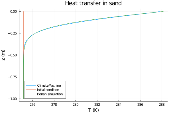

The plot shows that the temperature at the top of the soil is gradually increasing. This is because the surface temperature is held fixed at a value larger than the initial temperature. If we ran this for longer, we would see that the bottom of the domain would also increase in temperature because there is no heat leaving the bottom (due to zero heat flux specified in the boundary condition).

References

• G. Bonan (2019)
• O. Johanson (1977)
• V. Balland , P. A. Arp (2005)
• Yongjiu Dai al. (2019)
• B.J. Cosby al. (1984)

This page was generated using Literate.jl.