Hydraulic functions
This tutorial shows how to specify the hydraulic functions used in Richard's equation. In particular, we show how to choose the formalism for matric potential and hydraulic conductivity, and how to make the hydraulic conductivity account for the presence of ice as well as the temperature dependence of the viscosity of liquid water.
Preliminary setup
External modules
using PlotsClimateMachine modules
using ClimateMachine
using ClimateMachine.Land
using ClimateMachine.Land.SoilWaterParameterizations

FT = Float32;
Specifying a hydraulics model
ClimateMachine's Land model allows the user to pick between two hydraulics models, that of van Genuchten M. Th. Genuchten (1980) or that of Brooks and Corey, see R. J. Brooks , A. T. Corey (1964) or A. T. Corey (1977). The same model is consistently used for the matric potential and hydraulic conductivity.
The van Genuchten model requires two free parameters, α and n. A third parameter, m, is computed from n. Of these, only α carries units, of inverse meters. The Brooks and Corey model also uses two free parameters, ψ_b, the magnitude of the matric potential at saturation, and a constant M. ψ_b carries units of meters. These parameter sets are stored in either the vanGenuchten or the BrooksCorey hydraulics model structures (more details below). These parameters are enough to compute the matric potential.
The hydraulic conductivity requires an additional parameter, Ksat (m/s), which is the hydraulic conductivity in saturated soil. This parameter is not stored in the hydraulics model, but rather as part of the WaterParamFunctions, which stores other parameters needed for the soil water modeling.
Below we show how to create two concrete examples of these hydraulics models, for sandy loam (G. Bonan (2019)). Note that the parameters chosen are a function of soil type, and that the parameters are converted to type FT internally.
vg_α = 7.5 # m^-1
vg_n = 1.89
hydraulics = vanGenuchten(FT; α = vg_α, n = vg_n);

ψ_sat = 0.218 # m
Mval = 0.2041
hydraulics_bc = BrooksCorey(FT; ψb = ψ_sat, m = Mval);
Matric Potential
The matric potential ψ reflects the negative pressure of water in unsaturated soil. The negative pressure (suction) of water arises because of adhesive forces between water and soil.
The van Genuchten expression for matric potential is $ψ = -\frac{1}{α} S_l^{-1/(nm)}\times (1-S_l^{1/m})^{1/n},$
and the Brooks and Corey expression is $ψ = -ψ_b S_l^{-M}.$
Here S_l is the effective saturation of liquid water, θ_l/ν, where ν is porosity of the soil. We generally neglect the residual pore space in the CliMA model, but the user can set the parameter in the WaterParamFunctions structure if it is desired.
In the CliMA code, we use multiple dispatch. With multiple dispatch, a function can have many ways of executing (called methods), depending on the type of the variables passed in. A simple example of multiple dispatch is the division operation. Integer division takes two numbers as input, and returns an integer - ignoring the decimal. Float division takes two numbers as input, and returns a floating point number, including the decimal. In Julia, we might write these as:
function division(a::Int, b::Int)
     return floor(Int, a/b)
end
function division(a::Float64, b::Float64)
return a/b
endWe can see that division is now a function with two methods.
julia> division
division (generic function with 2 methods)
Now, using the same function signature, we can carry out integer division or floating point division, depending on the types of the arguments:
julia> division(1,2)
0

julia> division(1.0,2.0)
0.5
Here are more pertinent examples: Based on our choice of FT = Float32,
julia> typeof(hydraulics)
vanGenuchten{Float32,Float32,Float32,Float32}
but meanwhile,
julia> typeof(hydraulics_bc)
BrooksCorey{Float32,Float32,Float32}
The function matric_potential will execute different methods depending on if we pass a hydraulics model of type vanGenuchten or BrooksCorey. In both cases, it will return the correct value for ψ.
Let's plot the matric potential as a function of the effective saturation S_l = θ_l/ν, which can range from zero to one.
S_l = FT.(0.01:0.01:0.99)
ψ = matric_potential.(Ref(hydraulics), S_l)
ψ_bc = matric_potential.(Ref(hydraulics_bc), S_l)
plot(
    S_l,
    log10.(-ψ),
    xlabel = "effective saturation",
    ylabel = "Log10(|ψ|)",
    label = "van Genuchten",
)
plot!(S_l, log10.(-ψ_bc), label = "Brooks and Corey")
savefig("bc_vg_matric_potential.png")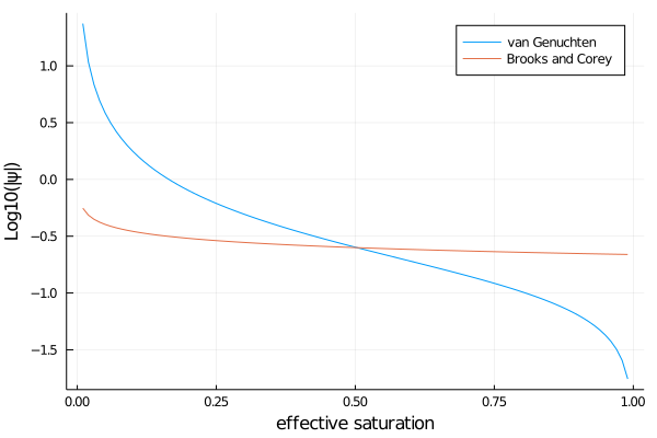
The steep slope in ψ near saturated and completely dry soil are part of the reason why Richard's equation is such a challenging numerical problem.
Hydraulic conductivity
The hydraulic conductivity is a more complex function than the matric potential, as it depends on the temperature of the water, the volumetric ice fraction, and the volumetric liquid water fraction. It also depends on the hydraulics model chosen.
We represent the hydraulic conductivity K as the product of four factors: Ksat, an impedance factor (which accounts for the effect of ice on conductivity) a viscosity factor (which accounts for the effect of temperature on the viscosity of liquid water, and how that in turn affects conductivity) and a moisture factor (which accounts for the effect of liquid water, and is determined by the hydraulics model). We are going to calculate K = Ksat × viscosity factor × impedance factor × moisture factor. In the code, each of these factors is computed by a function with multiple methods, except for Ksat. Like we defined new type classes for vanGenuchten and BrooksCorey, we also created new type classes for the impedance choice, the viscosity choice, and the moisture choice.
The function viscosity_factor takes as arguments the temperature of the soil and the viscosity model desired, and returns the factor k_v by which the hydraulic conductivity is scaled. One option is to account for this effect:
$k_v = e^{γ (T-T_{\rm ref})}$
where γ = 0.0264/K and $T_{\rm ref}$ = 288K.
For example, at the freezing point of water, using the default values for γ and T_ref, viscosity reduces the conductivity by a third:
viscous_effect_model = TemperatureDependentViscosity{FT}();
viscosity_factor(viscous_effect_model, FT(273.15))0.67567694f0The other option is to ignore this effect:
$k_v = 1$
This is the default approach.
no_viscous_effect_model = ConstantViscosity{FT}();
viscosity_factor(no_viscous_effect_model, FT(273.15))1.0f0Very similarly, the function impedance_factor takes as arguments the liquid water and ice volumetric fractions in the soil, as well as the impedance model being used, and returns the factor k_i by which the hydraulic conductivity is scaled. One option is to account for this effect:
$k_i = 10^{-Ω f_i},$
where Ω = 7 is an empirical factor and f_i is the ratio of the volumetric ice fraction to total volumetric water fraction (L.C. Lundin (1990)).
For example, with $\theta_i = \theta_l$, or f_i = 0.5, ice reduces the conductivity by over 1000x.
impedance_effect_model = IceImpedance{FT}();
impedance_factor(impedance_effect_model, FT(0.5))0.00031622776f0The other option is to ignore this effect:
$k_i = 1$
This is the default approach.
no_impedance_effect_model = NoImpedance{FT}();
impedance_factor(no_impedance_effect_model, FT(0.5))1.0f0As for the moisture dependence of hydraulic conductivity, it can also be either independent of moisture, or dependent on moisture. If it is dependent on moisture, the specific function evaluated is dictated by the hydraulics model. The moisture_factor for the van Genuchten model is (denoting it as $k_m$)
$k_m = \sqrt{S_l}[1-(1-S_l^{1/m})^m]^2,$
for $S_l < 1$,
and for the Brooks and Corey model it is
$k_m = S_l^{2M+3},$
also for $S_l<1$. When $S_l\geq 1$, $k_m = 1$ for each model.
Let's put all these factors together now. Below we choose additional parameters, consistent with the hydraulics parameters for sandy loam (G. Bonan (2019)), and show how hydraulic conductivity varies with liquid water content, in the case without ice impedance or temperature effects.
Ksat = FT(4.42 / (3600 * 100))
T = FT(0.0)
f_i = FT(0.0)
K =
    hydraulic_conductivity.(
        Ref(Ksat),
        Ref(impedance_factor(NoImpedance{FT}(), f_i)),
        Ref(viscosity_factor(ConstantViscosity{FT}(), T)),
        moisture_factor.(Ref(MoistureDependent{FT}()), Ref(hydraulics), S_l),
    );
Let's also compute K when we include the effects of temperature and ice on the hydraulic conductivity. In the cases where a TemperatureDependentViscosity or IceImpedance type is passed, the correct factors are calculated, based on the temperature T and volumetric ice fraction θ_i.
T = FT(273.15)
S_i = FT(0.1); # = θ_i/ν
The total volumetric water fraction cannot exceed unity, so the effective liquid water saturation should have a max of 1-S_i.
S_l_accounting_for_ice = FT.(0.01:0.01:(0.99 - S_i))
f_i = S_i ./ (S_l_accounting_for_ice .+ S_i)
K_w_factors =
    hydraulic_conductivity.(
        Ref(Ksat),
        impedance_factor.(Ref(NoImpedance{FT}()), f_i),
        Ref(viscosity_factor(ConstantViscosity{FT}(), T)),
        moisture_factor.(
            Ref(MoistureDependent{FT}()),
            Ref(hydraulics),
            S_l_accounting_for_ice,
        ),
    );
plot(
    S_l,
    log10.(K),
    xlabel = "total effective saturation, (θ_i+θ_l)/ν",
    ylabel = "Log10(K)",
    label = "Base case",
    legend = :bottomright,
)
plot!(
    S_l_accounting_for_ice .+ S_i,
    log10.(K_w_factors),
    label = "θ_i = 0.1, T = 273.15",
)
savefig("T_ice_K.png")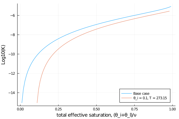
If the user is not considering phase transitions and does not add in Freeze/Thaw source terms, the default is for zero ice in the model, for all time and space. In this case the ice impedance factor evaluates to 1 regardless of which type is passed.
Other features
The user also has the choice of making the conductivity constant by choosing MoistureIndependent along with ConstantViscosity and NoImpedance. This is useful for debugging!
no_moisture_dependence = MoistureIndependent{FT}()
K_constant =
    hydraulic_conductivity.(
        Ref(Ksat),
        Ref(FT(1.0)),
        Ref(FT(1.0)),
        moisture_factor.(Ref(no_moisture_dependence), Ref(hydraulics), S_l),
    );
julia> unique(K_constant)
1-element Array{Float32,1}:
1.2277777f-5Note that choosing this option does not mean the matric potential is constant, as a hydraulics model is still required and employed.
And, lastly, you might also find it helpful in debugging to be able to turn off the flow of water by setting Ksat = 0.
References
- M. Th. Genuchten (1980)
- R. J. Brooks , A. T. Corey (1964)
- A. T. Corey (1977)
- L.C. Lundin (1990)
- G. Bonan (2019)
This page was generated using Literate.jl.