Batched Generalized Minimal Residual
In this tutorial we describe the basics of using the batched gmres iterative solver. At the end you should be able to
- Use BatchedGeneralizedMinimalResidual to solve batches of linear systems
- Construct a columnwise linear solver with BatchedGeneralizedMinimalResidual
What is the Generalized Minimal Residual Method?
The Generalized Minimal Residual Method (GMRES) is a Krylov subspace method for solving linear systems:
\[ Ax = b\]
See the wikipedia for more details.
What is the Batched Generalized Minimal Residual Method?
As the name suggests it solves a whole bunch of independent GMRES problems
Basic Example
First we must load a few things
using ClimateMachine
using ClimateMachine.SystemSolvers
using LinearAlgebra, Random, Plots
Next we define two linear systems that we would like to solve simultaneously. The matrix for the first linear system is
A1 = [
    2.0 -1.0 0.0
    -1.0 2.0 -1.0
    0.0 -1.0 2.0
];
And the right hand side is
b1 = ones(typeof(1.0), 3);The exact solution to the first linear system is
x1_exact = [1.5, 2.0, 1.5];The matrix for the first linear system is
A2 = [
    2.0 -1.0 0.0
    0.0 2.0 -1.0
    0.0 0.0 2.0
];
And the right hand side is
b2 = ones(typeof(1.0), 3);The exact solution to second linear system is
x2_exact = [0.875, 0.75, 0.5];We now define a function that performs the action of each linear operator independently.
function closure_linear_operator(A1, A2)
    function linear_operator!(x, y)
        mul!(view(x, :, 1), A1, view(y, :, 1))
        mul!(view(x, :, 2), A2, view(y, :, 2))
        return nothing
    end
    return linear_operator!
end;
To understand how this works let us construct an instance of the linear operator and apply it to a vector
linear_operator! = closure_linear_operator(A1, A2);Let us see what the action of this linear operator is
y1 = ones(typeof(1.0), 3);
y2 = ones(typeof(1.0), 3) * 2.0;
y = [y1 y2];
x = copy(y);
linear_operator!(x, y);
x
3×2 Array{Float64,2}:
1.0 2.0
0.0 2.0
1.0 4.0We see that the first column is A1 * [1 1 1]' and the second column is A2 * [2 2 2]' that is,
[A1 * y1 A2 * y2]3×2 Array{Float64,2}:
1.0 2.0
0.0 2.0
1.0 4.0We are now ready to set up our Batched Generalized Minimal Residual solver We must now set up the right hand side of the linear system
b = [b1 b2];as well as the exact solution, (to verify convergence)
x_exact = [x1_exact x2_exact];For BatchedGeneralizedMinimalResidual the assumption is that each column of b is independent and corresponds to a batch. This will come back later.
We now use an instance of the solver
linearsolver = BatchedGeneralizedMinimalResidual(b, size(A1, 1), 2);As well as an initial guess, denoted by the variable x
x1 = ones(typeof(1.0), 3);
x2 = ones(typeof(1.0), 3);
x = [x1 x2];
To solve the linear system, we just need to pass to the linearsolve! function
iters = linearsolve!(linear_operator!, nothing, linearsolver, x, b)3which is guaranteed to converge in 3 iterations since length(b1)=length(b2)=3 We can now check that the solution that we computed, x
x3×2 Array{Float64,2}:
1.5 0.875
2.0 0.75
1.5 0.5has converged to the exact solution
x_exact3×2 Array{Float64,2}:
1.5 0.875
2.0 0.75
1.5 0.5Which indeed it has.
Advanced Example
We now go through a more advanced application of the Batched Generalized Minimal Residual solver
Iterative methods should be used with preconditioners!
The first thing we do is define a linear operator that mimics the behavior of a columnwise operator in ClimateMachine
function closure_linear_operator!(A, tup)
    function linear_operator!(y, x)
        alias_x = reshape(x, tup)
        alias_y = reshape(y, tup)
        for i6 in 1:tup[6]
            for i4 in 1:tup[4]
                for i2 in 1:tup[2]
                    for i1 in 1:tup[1]
                        tmp = alias_x[i1, i2, :, i4, :, i6][:]
                        tmp2 = A[i1, i2, i4, i6] * tmp
                        alias_y[i1, i2, :, i4, :, i6] .=
                            reshape(tmp2, (tup[3], tup[5]))
                    end
                end
            end
        end
    end
end;
Next we define the array structure of an MPIStateArray in its true high dimensional form
tup = (2, 2, 5, 2, 10, 2);We define our linear operator as a random matrix
Random.seed!(1234);
B = [
    randn(tup[3] * tup[5], tup[3] * tup[5])
    for i1 in 1:tup[1], i2 in 1:tup[2], i4 in 1:tup[4], i6 in 1:tup[6]
];
columnwise_A = [
    B[i1, i2, i4, i6] + 3 * (i1 + i2 + i4 + i6) * I
    for i1 in 1:tup[1], i2 in 1:tup[2], i4 in 1:tup[4], i6 in 1:tup[6]
];
as well as its inverse
columnwise_inv_A = [
    inv(columnwise_A[i1, i2, i4, i6])
    for i1 in 1:tup[1], i2 in 1:tup[2], i4 in 1:tup[4], i6 in 1:tup[6]
];
columnwise_linear_operator! = closure_linear_operator!(columnwise_A, tup);
columnwise_inverse_linear_operator! =
    closure_linear_operator!(columnwise_inv_A, tup);
The structure of an MPIStateArray is related to its true higher dimensional form as follows:
mpi_tup = (tup[1] * tup[2] * tup[3], tup[4], tup[5] * tup[6]);We now define the right hand side of our Linear system
b = randn(mpi_tup);As well as the initial guess
x = copy(b);
x += randn(mpi_tup) * 0.1;
In the previous tutorial we mentioned that it is assumed that the right hand side is an array whose column vectors all independent linear systems. But right now the array structure of $x$ and $b$ do not follow this requirement. To handle this case we must pass in additional arguments that tell the linear solver how to reconcile these differences. The first thing that the linear solver must know of is the higher tensor form of the MPIStateArray, which is just the tup from before
reshape_tuple_f = tup;The second thing it needs to know is which indices correspond to a column and we want to make sure that these are the first set of indices that appear in the permutation tuple (which can be thought of as enacting a Tensor Transpose).
permute_tuple_f = (5, 3, 4, 6, 1, 2);It has this format since the 3 and 5 index slots are the ones associated with traversing a column. And the 4 index slot corresponds to a state. We also need to tell our solver which kind of Array struct to use
ArrayType = Array;We are now ready to finally define our linear solver, which uses a number of keyword arguments
gmres = BatchedGeneralizedMinimalResidual(
    b,
    tup[3] * tup[5] * tup[4],
    tup[1] * tup[2] * tup[6];
    atol = eps(Float64) * 100,
    rtol = eps(Float64) * 100,
    forward_reshape = reshape_tuple_f,
    forward_permute = permute_tuple_f,
);
m is the number of gridpoints along a column. As mentioned previously, this is tup[3]*tup[5]*tup[4]. The n term corresponds to the batch size or the number of columns in this case. atol and rtol are relative and absolute tolerances
All the hard work is done, now we just call our linear solver
iters = linearsolve!(
    columnwise_linear_operator!,
    nothing,
    gmres,
    x,
    b,
    max_iters = tup[3] * tup[5] * tup[4],
)52We see that it converged in less than tup[3]*tup[5] = 50 iterations. Let us verify that it is indeed correct by computing the exact answer numerically and comparing it against the iterative solver.
x_exact = copy(x);
columnwise_inverse_linear_operator!(x_exact, b);
Now we can compare with some norms
norm(x - x_exact) / norm(x_exact)
columnwise_linear_operator!(x_exact, x);
norm(x_exact - b) / norm(b)1.2827339696812677e-13Which we see are small, given our choice of atol and rtol. The struct also keeps a record of its convergence rate in the residual member (max over all batched solvers). The can be visualized via
plot(log.(gmres.resnorms[:]) / log(10));
plot!(legend = false, xlims = (1, iters), ylims = (-15, 2));
plot!(ylabel = "log10 residual", xlabel = "iterations")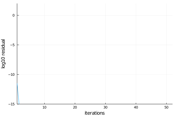
This page was generated using Literate.jl.