Coupled heat and water equations tending towards equilibrium

Other tutorials, such as the soil heat tutorial and Richards equation tutorial demonstrate how to solve the heat equation or Richard's equation without considering dynamic interactions between the two. As an example, the user could prescribe a fixed function of space and time for the liquid water content, and use that to drive the heat equation, but without allowing the water content to dynamically evolve according to Richard's equation and without allowing the changing temperature of the soil to affect the water evolution.

Here we show how to solve the interacting heat and water equations, in sand, but without phase changes. This allows us to capture behavior that is not present in the decoupled equations.

The equations are:

$\frac{∂ ρe_{int}}{∂ t} = ∇ ⋅ κ(θ_l, θ_i; ν, ...) ∇T + ∇ ⋅ ρe_{int_{liq}} K (T,θ_l, θ_i; ν, ...) \nabla h( ϑ_l, z; ν, ...)$

$\frac{ ∂ ϑ_l}{∂ t} = ∇ ⋅ K (T,θ_l, θ_i; ν, ...) ∇h( ϑ_l, z; ν, ...).$

Here

$t$ is the time (s),

$z$ is the location in the vertical (m),

$ρe_{int}$ is the volumetric internal energy of the soil (J/m^3),

$T$ is the temperature of the soil (K),

$κ$ is the thermal conductivity (W/m/K),

$ρe_{int_{liq}}$ is the volumetric internal energy of liquid water (J/m^3),

$K$ is the hydraulic conductivity (m/s),

$h$ is the hydraulic head (m),

$ϑ_l$ is the augmented volumetric liquid water fraction,

$θ_i$ is the volumetric ice fraction, and

$ν, ...$ denotes parameters relating to soil type, such as porosity.

We will solve this equation in an effectively 1-d domain with $z ∈ [-1,0]$, and with the following boundary and initial conditions:

$- κ ∇T(t, z = 0) = 0 ẑ$

$-κ ∇T(t, z = -1) = 0 ẑ$

$T(t = 0, z) = T_{min} + (T_{max}-T_{min}) e^{Cz}$

$- K ∇h(t, z = 0) = 0 ẑ$

$-K ∇h(t, z = -1) = 0 ẑ$

$ϑ(t = 0, z) = ϑ_{min} + (ϑ_{max}-ϑ_{min}) e^{Cz},$

where $C, T_{min}, T_{max}, ϑ_{min},$ and $ϑ_{max}$ are constants.

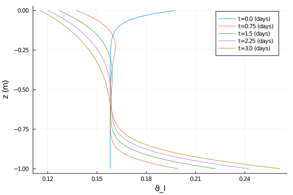
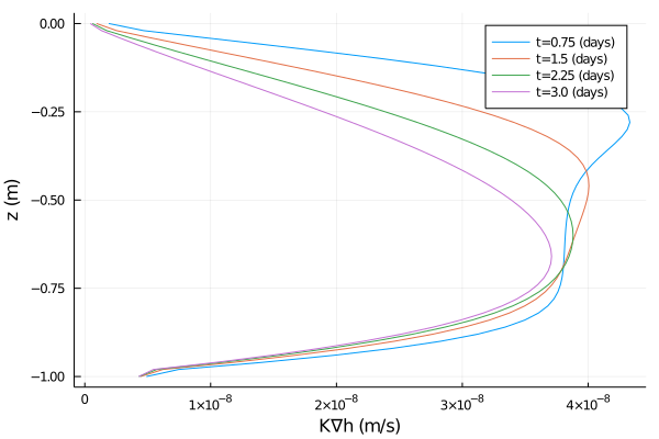
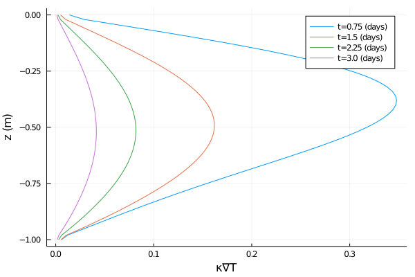
If we evolve this system for times long compared to the dynamical timescales of the system, we expect it to reach an equilibrium where the LHS of these equations tends to zero. Assuming zero fluxes at the boundaries, the resulting equilibrium state should satisfy $∂h/∂z = 0$ and $∂T/∂z = 0$. Physically, this means that the water settles into a vertical profile in which the resulting pressure balances gravity and that the temperature is constant across the domain.

We verify that the system is approaching this equilibrium, and we also sketch out an analytic calculation for the final temperature in equilibrium.

Import necessary modules

External (non - CliMA) modules

using MPI
using OrderedCollections
using StaticArrays
using Statistics
using Plots

CliMA Parameters

using CLIMAParameters
using CLIMAParameters.Planet: ρ_cloud_liq, ρ_cloud_ice, cp_l, cp_i, T_0, LH_f0

ClimateMachine modules

using ClimateMachine
using ClimateMachine.Land
using ClimateMachine.Land.SoilWaterParameterizations
using ClimateMachine.Land.SoilHeatParameterizations
using ClimateMachine.Mesh.Topologies
using ClimateMachine.Mesh.Grids
using ClimateMachine.Diagnostics
using ClimateMachine.ConfigTypes
using ClimateMachine.DGMethods
using ClimateMachine.DGMethods.NumericalFluxes
using ClimateMachine.DGMethods: BalanceLaw, LocalGeometry
using ClimateMachine.MPIStateArrays
using ClimateMachine.GenericCallbacks
using ClimateMachine.ODESolvers
using ClimateMachine.VariableTemplates
using ClimateMachine.SingleStackUtils
using ClimateMachine.BalanceLaws:
    BalanceLaw,
    Prognostic,
    Auxiliary,
    Gradient,
    GradientFlux,
    vars_state,
    parameter_set

Preliminary set-up

Get the parameter set, which holds constants used across CliMA models:

struct EarthParameterSet <: AbstractEarthParameterSet end
const param_set = EarthParameterSet();

Initialize and pick a floating point precision:

ClimateMachine.init()
const FT = Float64;

Load plot helpers:

const clima_dir = dirname(dirname(pathof(ClimateMachine)));
include(joinpath(clima_dir, "docs", "plothelpers.jl"));

Set soil parameters to be consistent with sand. Please see e.g. the soil heat tutorial for other soil type parameters, or B.J. Cosby al. (1984).

The porosity:

porosity = FT(0.395);

Soil solids are the components of soil besides water, ice, gases, and air. We specify the soil component fractions, relative to all soil solids. These should sum to unity; they do not account for pore space.

ν_ss_quartz = FT(0.92)
ν_ss_minerals = FT(0.08)
ν_ss_om = FT(0.0)
ν_ss_gravel = FT(0.0);

Other parameters include the hydraulic conductivity at saturation, the specific storage, and the van Genuchten parameters for sand. We recommend Chapter 8 of G. Bonan (2019) for finding parameters for other soil types.

Ksat = FT(4.42 / 3600 / 100) # m/s
S_s = FT(1e-3) #inverse meters
vg_n = FT(1.89)
vg_α = FT(7.5); # inverse meters

Other constants needed:

κ_quartz = FT(7.7) # W/m/K
κ_minerals = FT(2.5) # W/m/K
κ_om = FT(0.25) # W/m/K
κ_liq = FT(0.57) # W/m/K
κ_ice = FT(2.29); # W/m/K

The particle density of organic material-free soil is equal to the particle density of quartz and other minerals (V. Balland , P. A. Arp (2005)):

ρp = FT(2700); # kg/m^3

We calculate the thermal conductivities for the solid material and for saturated soil. These functions are taken from V. Balland , P. A. Arp (2005).

κ_solid = k_solid(ν_ss_om, ν_ss_quartz, κ_quartz, κ_minerals, κ_om)
κ_sat_frozen = ksat_frozen(κ_solid, porosity, κ_ice)
κ_sat_unfrozen = ksat_unfrozen(κ_solid, porosity, κ_liq);

Next, we calculate the volumetric heat capacity of dry soil. Dry soil refers to soil that has no water content.

ρc_ds = FT((1 - porosity) * 1.926e06); # J/m^3/K

We collect the majority of the parameters needed for modeling heat and water flow in soil in soil_param_functions, an object of type SoilParamFunctions. Parameters used only for hydrology are stored in water, which is of type WaterParamFunctions.

soil_param_functions = SoilParamFunctions(
    FT;
    porosity = porosity,
    ν_ss_gravel = ν_ss_gravel,
    ν_ss_om = ν_ss_om,
    ν_ss_quartz = ν_ss_quartz,
    ρc_ds = ρc_ds,
    ρp = ρp,
    κ_solid = κ_solid,
    κ_sat_unfrozen = κ_sat_unfrozen,
    κ_sat_frozen = κ_sat_frozen,
    water = WaterParamFunctions(FT; Ksat = Ksat, S_s = S_s),
);

Initial and Boundary conditions

As we are not including the equations for phase changes in this tutorial, we chose temperatures that are above the freezing point of water.

The initial temperature profile:

function T_init(aux)
    FT = eltype(aux)
    zmax = FT(0)
    zmin = FT(-1)
    T_max = FT(289.0)
    T_min = FT(288.0)
    c = FT(20.0)
    z = aux.z
    output = T_min + (T_max - T_min) * exp(-(z - zmax) / (zmin - zmax) * c)
    return output
end;

The initial water profile:

function ϑ_l0(aux)
    FT = eltype(aux)
    zmax = FT(0)
    zmin = FT(-1)
    theta_max = FT(porosity * 0.5)
    theta_min = FT(porosity * 0.4)
    c = FT(20.0)
    z = aux.z
    output =
        theta_min +
        (theta_max - theta_min) * exp(-(z - zmax) / (zmin - zmax) * c)
    return output
end;

The boundary value problem in this case requires a boundary condition at the top and the bottom of the domain for each equation being solved. These conditions can be Dirichlet, or Neumann.

Dirichlet boundary conditions are on ϑ_l and T, while Neumann boundary conditions are on -κ∇T and -K∇h. For Neumann conditions, the user supplies a scalar, which is multiplied by ẑ within the code.

Water boundary conditions:

surface_water_flux = (aux, t) -> eltype(aux)(0.0)
bottom_water_flux = (aux, t) -> eltype(aux)(0.0);

The boundary conditions for the heat equation:

surface_heat_flux = (aux, t) -> eltype(aux)(0.0)
bottom_heat_flux = (aux, t) -> eltype(aux)(0.0);

bc = LandDomainBC(
    bottom_bc = LandComponentBC(
        soil_heat = Neumann(bottom_heat_flux),
        soil_water = Neumann(bottom_water_flux),
    ),
    surface_bc = LandComponentBC(
        soil_heat = Neumann(surface_heat_flux),
        soil_water = Neumann(surface_water_flux),
    ),
);

Next, we define the required init_soil! function, which takes the user specified functions of space for T_init and ϑ_l0 and initializes the state variables of volumetric internal energy and augmented liquid fraction. This requires a conversion from T to ρe_int.

function init_soil!(land, state, aux, localgeo, time)
    myFT = eltype(state)
    ϑ_l = myFT(land.soil.water.initialϑ_l(aux))
    θ_i = myFT(land.soil.water.initialθ_i(aux))
    state.soil.water.ϑ_l = ϑ_l
    state.soil.water.θ_i = θ_i
    param_set = parameter_set(land)

    θ_l = volumetric_liquid_fraction(ϑ_l, land.soil.param_functions.porosity)
    ρc_ds = land.soil.param_functions.ρc_ds
    ρc_s = volumetric_heat_capacity(θ_l, θ_i, ρc_ds, param_set)

    state.soil.heat.ρe_int = volumetric_internal_energy(
        θ_i,
        ρc_s,
        land.soil.heat.initialT(aux),
        param_set,
    )
end;

Create the soil model structure

First, for water (this is where the hydrology parameters are supplied):

soil_water_model = SoilWaterModel(
    FT;
    viscosity_factor = TemperatureDependentViscosity{FT}(),
    moisture_factor = MoistureDependent{FT}(),
    hydraulics = vanGenuchten(FT; α = vg_α, n = vg_n),
    initialϑ_l = ϑ_l0,
);

Note that the viscosity of water depends on temperature. We account for the effect that has on the hydraulic conductivity by specifying viscosity_factor = TemperatureDependentViscosity{FT}(). The default, if no viscosity_factor keyword argument is supplied, is to not include the effect of T on viscosity. More guidance about specifying the hydraulic conductivity, and the hydraulics model, can be found in the hydraulic functions tutorial.

Repeat for heat:

soil_heat_model = SoilHeatModel(FT; initialT = T_init)

ClimateMachine.Land.SoilHeatModel{Float64,typeof(Main.##392.T_init)}(Main.##392.T_init)

Combine into a single soil model:

m_soil = SoilModel(soil_param_functions, soil_water_model, soil_heat_model);

We aren't using any sources or sinks in the equations here, but this is where freeze/thaw terms, runoff, root extraction, etc. would go.

sources = ();

Create the LandModel - without other components (canopy, carbon, etc):

m = LandModel(
    param_set,
    m_soil;
    boundary_conditions = bc,
    source = sources,
    init_state_prognostic = init_soil!,
);

Specify the numerical details

Choose a resolution, domain boundaries, integration time, timestep, and ODE solver.

N_poly = 1
nelem_vert = 50
zmin = FT(-1)
zmax = FT(0)

driver_config = ClimateMachine.SingleStackConfiguration(
    "LandModel",
    N_poly,
    nelem_vert,
    zmax,
    param_set,
    m;
    zmin = zmin,
    numerical_flux_first_order = CentralNumericalFluxFirstOrder(),
)

t0 = FT(0)
timeend = FT(60 * 60 * 72)
dt = FT(30.0)


solver_config =
    ClimateMachine.SolverConfiguration(t0, timeend, driver_config, ode_dt = dt);

ClimateMachine.array_type() = Array
┌ Info: Model composition
│     param_set = Main.##392.EarthParameterSet()
│     soil = ClimateMachine.Land.SoilModel{ClimateMachine.Land.SoilParamFunctions{Float64,Float64,Float64,Float64,Float64,Float64,Float64,Float64,Float64,Float64,Float64,Float64,Float64,ClimateMachine.Land.WaterParamFunctions{Float64,ClimateMachine.Land.var"#3#15"{Float64,Float64},ClimateMachine.Land.var"#5#17"{Float64,Float64},ClimateMachine.Land.var"#8#20"{Float64,ClimateMachine.Land.var"#14#26"}}},ClimateMachine.Land.SoilWaterModel{Float64,ClimateMachine.Land.SoilWaterParameterizations.NoImpedance{Float64},ClimateMachine.Land.SoilWaterParameterizations.TemperatureDependentViscosity{Float64},ClimateMachine.Land.SoilWaterParameterizations.MoistureDependent{Float64},ClimateMachine.Land.SoilWaterParameterizations.vanGenuchten{Float64,Float64,Float64,Float64},typeof(Main.##392.ϑ_l0),ClimateMachine.Land.var"#38#42"},ClimateMachine.Land.SoilHeatModel{Float64,typeof(Main.##392.T_init)}}(ClimateMachine.Land.SoilParamFunctions{Float64,Float64,Float64,Float64,Float64,Float64,Float64,Float64,Float64,Float64,Float64,Float64,Float64,ClimateMachine.Land.WaterParamFunctions{Float64,ClimateMachine.Land.var"#3#15"{Float64,Float64},ClimateMachine.Land.var"#5#17"{Float64,Float64},ClimateMachine.Land.var"#8#20"{Float64,ClimateMachine.Land.var"#14#26"}}}(0.395, 0.0, 0.0, 0.92, 1.16523e6, 2700.0, 7.037309762302548, 2.6076638236870164, 4.516645961171465, 0.24, 18.1, 0.053, ClimateMachine.Land.WaterParamFunctions{Float64,ClimateMachine.Land.var"#3#15"{Float64,Float64},ClimateMachine.Land.var"#5#17"{Float64,Float64},ClimateMachine.Land.var"#8#20"{Float64,ClimateMachine.Land.var"#14#26"}}(ClimateMachine.Land.var"#3#15"{Float64,Float64}(1.2277777777777777e-5), ClimateMachine.Land.var"#5#17"{Float64,Float64}(0.001), ClimateMachine.Land.var"#8#20"{Float64,ClimateMachine.Land.var"#14#26"}(ClimateMachine.Land.var"#14#26"()))), ClimateMachine.Land.SoilWaterModel{Float64,ClimateMachine.Land.SoilWaterParameterizations.NoImpedance{Float64},ClimateMachine.Land.SoilWaterParameterizations.TemperatureDependentViscosity{Float64},ClimateMachine.Land.SoilWaterParameterizations.MoistureDependent{Float64},ClimateMachine.Land.SoilWaterParameterizations.vanGenuchten{Float64,Float64,Float64,Float64},typeof(Main.##392.ϑ_l0),ClimateMachine.Land.var"#38#42"}(ClimateMachine.Land.SoilWaterParameterizations.NoImpedance{Float64}(), ClimateMachine.Land.SoilWaterParameterizations.TemperatureDependentViscosity{Float64}(0.0264, 288.0), ClimateMachine.Land.SoilWaterParameterizations.MoistureDependent{Float64}(), ClimateMachine.Land.SoilWaterParameterizations.vanGenuchten{Float64,Float64,Float64,Float64}(1.89, 7.5, 0.4708994708994708), Main.##392.ϑ_l0, ClimateMachine.Land.var"#38#42"()), ClimateMachine.Land.SoilHeatModel{Float64,typeof(Main.##392.T_init)}(Main.##392.T_init))
│     surface = ClimateMachine.Land.SurfaceFlow.NoSurfaceFlowModel()
│     boundary_conditions = ClimateMachine.Land.LandDomainBC{ClimateMachine.Land.LandComponentBC{ClimateMachine.Land.Neumann{Main.##392.var"#11#12"},ClimateMachine.Land.Neumann{Main.##392.var"#15#16"},ClimateMachine.Land.NoBC},ClimateMachine.Land.LandComponentBC{ClimateMachine.Land.Neumann{Main.##392.var"#13#14"},ClimateMachine.Land.Neumann{Main.##392.var"#17#18"},ClimateMachine.Land.NoBC},ClimateMachine.Land.LandComponentBC{ClimateMachine.Land.NoBC,ClimateMachine.Land.NoBC,ClimateMachine.Land.NoBC},ClimateMachine.Land.LandComponentBC{ClimateMachine.Land.NoBC,ClimateMachine.Land.NoBC,ClimateMachine.Land.NoBC},ClimateMachine.Land.LandComponentBC{ClimateMachine.Land.NoBC,ClimateMachine.Land.NoBC,ClimateMachine.Land.NoBC},ClimateMachine.Land.LandComponentBC{ClimateMachine.Land.NoBC,ClimateMachine.Land.NoBC,ClimateMachine.Land.NoBC}}(ClimateMachine.Land.LandComponentBC{ClimateMachine.Land.Neumann{Main.##392.var"#11#12"},ClimateMachine.Land.Neumann{Main.##392.var"#15#16"},ClimateMachine.Land.NoBC}(ClimateMachine.Land.Neumann{Main.##392.var"#11#12"}(Main.##392.var"#11#12"()), ClimateMachine.Land.Neumann{Main.##392.var"#15#16"}(Main.##392.var"#15#16"()), ClimateMachine.Land.NoBC()), ClimateMachine.Land.LandComponentBC{ClimateMachine.Land.Neumann{Main.##392.var"#13#14"},ClimateMachine.Land.Neumann{Main.##392.var"#17#18"},ClimateMachine.Land.NoBC}(ClimateMachine.Land.Neumann{Main.##392.var"#13#14"}(Main.##392.var"#13#14"()), ClimateMachine.Land.Neumann{Main.##392.var"#17#18"}(Main.##392.var"#17#18"()), ClimateMachine.Land.NoBC()), ClimateMachine.Land.LandComponentBC{ClimateMachine.Land.NoBC,ClimateMachine.Land.NoBC,ClimateMachine.Land.NoBC}(ClimateMachine.Land.NoBC(), ClimateMachine.Land.NoBC(), ClimateMachine.Land.NoBC()), ClimateMachine.Land.LandComponentBC{ClimateMachine.Land.NoBC,ClimateMachine.Land.NoBC,ClimateMachine.Land.NoBC}(ClimateMachine.Land.NoBC(), ClimateMachine.Land.NoBC(), ClimateMachine.Land.NoBC()), ClimateMachine.Land.LandComponentBC{ClimateMachine.Land.NoBC,ClimateMachine.Land.NoBC,ClimateMachine.Land.NoBC}(ClimateMachine.Land.NoBC(), ClimateMachine.Land.NoBC(), ClimateMachine.Land.NoBC()), ClimateMachine.Land.LandComponentBC{ClimateMachine.Land.NoBC,ClimateMachine.Land.NoBC,ClimateMachine.Land.NoBC}(ClimateMachine.Land.NoBC(), ClimateMachine.Land.NoBC(), ClimateMachine.Land.NoBC()))
│     source = ()
│     source_dt = DispatchedTuples.DispatchedTuple{Tuple{},DispatchedTuples.NoDefaults} with 0 entries:
│   default => ()
│ 
│     init_state_prognostic = init_soil!
└ @ ClimateMachine /central/scratch/climaci/climatemachine-docs/1430/climatemachine-docs/src/Driver/driver_configs.jl:188
┌ Warning: This table is temporarily incomplete
└ @ ClimateMachine.BalanceLaws /central/scratch/climaci/climatemachine-docs/1430/climatemachine-docs/src/BalanceLaws/show_tendencies.jl:51

PDE: ∂_t Y_i + (∇•F_1(Y))_i + (∇•F_2(Y,G)))_i = (S(Y,G))_i
┌──────────────────────────┬──────────────────┬─────────────────────────────────────┬────────┐
│                 Equation │ Flux{FirstOrder} │                   Flux{SecondOrder} │ Source │
│                    (Y_i) │            (F_1) │                               (F_2) │    (S) │
├──────────────────────────┼──────────────────┼─────────────────────────────────────┼────────┤
│ VolumetricLiquidFraction │               () │                         (DarcyFlux) │     () │
│    VolumetricIceFraction │               () │                                  () │     () │
│ VolumetricInternalEnergy │               () │ (DiffHeatFlux, DarcyDrivenHeatFlux) │     () │
└──────────────────────────┴──────────────────┴─────────────────────────────────────┴────────┘

┌ Info: Establishing single stack configuration for LandModel
│     precision               = Float64
│     horiz polynomial order  = 1
│     vert polynomial order   = 1
│     domain_min              = 0.00 m, 0.00 m, -1.00 m
│     domain_max              = 1.00 m, 1.00 m, 0.00 m
│     # vert elems            = 50
│     MPI ranks               = 1
│     min(Δ_horz)             = 1.00 m
│     min(Δ_vert)             = 0.02 m
└ @ ClimateMachine /central/scratch/climaci/climatemachine-docs/1430/climatemachine-docs/src/Driver/driver_configs.jl:612
┌ Info: Initializing LandModel
└ @ ClimateMachine /central/scratch/climaci/climatemachine-docs/1430/climatemachine-docs/src/Driver/solver_configs.jl:185

Determine how often you want output:

const n_outputs = 4
const every_x_simulation_time = ceil(Int, timeend / n_outputs);

Store initial condition at $t=0$, including prognostic, auxiliary, and gradient flux variables:

state_types = (Prognostic(), Auxiliary(), GradientFlux())
dons_arr = Dict[dict_of_nodal_states(solver_config, state_types; interp = true)]
time_data = FT[0] # store time data

1-element Array{Float64,1}:
 0.0

We specify a function which evaluates every_x_simulation_time and returns the state vector, appending the variables we are interested in into dons_arr.

callback = GenericCallbacks.EveryXSimulationTime(every_x_simulation_time) do
    dons = dict_of_nodal_states(solver_config, state_types; interp = true)
    push!(dons_arr, dons)
    push!(time_data, gettime(solver_config.solver))
    nothing
end;

Run the integration

ClimateMachine.invoke!(solver_config; user_callbacks = (callback,));

┌ Info: Starting LandModel
│     dt              = 3.00000e+01
│     timeend         = 259200.00
│     number of steps = 8640
│     norm(Q)         = 2.7324714577227090e+07
└ @ ClimateMachine /central/scratch/climaci/climatemachine-docs/1430/climatemachine-docs/src/Driver/Driver.jl:802
┌ Info: Update
│     simtime = 219090.00 / 259200.00
│     wallclock = 00:01:00
│     efficiency (simtime / wallclock) = 3623.8980
│     wallclock end (estimated) = 00:01:11
│     norm(Q) = 2.7356151419399317e+07
└ @ ClimateMachine.Callbacks /central/scratch/climaci/climatemachine-docs/1430/climatemachine-docs/src/Driver/Callbacks/Callbacks.jl:75
┌ Info: Finished
│     norm(Q)            = 2.7369613412716899e+07
│     norm(Q) / norm(Q₀) = 1.0016431584440859e+00
│     norm(Q) - norm(Q₀) = 4.4898835489809513e+04
└ @ ClimateMachine /central/scratch/climaci/climatemachine-docs/1430/climatemachine-docs/src/Driver/Driver.jl:853

Get z-coordinate

z = get_z(solver_config.dg.grid; rm_dupes = true);

Let's export a plot of the initial state

output_dir = @__DIR__;

mkpath(output_dir);

export_plot(
    z,
    time_data ./ (60 * 60 * 24),
    dons_arr,
    ("soil.water.ϑ_l",),
    joinpath(output_dir, "eq_moisture_plot.png");
    xlabel = "ϑ_l",
    ylabel = "z (m)",
    time_units = "(days)",
)

export_plot(
    z,
    time_data[2:end] ./ (60 * 60 * 24),
    dons_arr[2:end],
    ("soil.water.K∇h[3]",),
    joinpath(output_dir, "eq_hydraulic_head_plot.png");
    xlabel = "K∇h (m/s)",
    ylabel = "z (m)",
    time_units = "(days)",
)

export_plot(
    z,
    time_data ./ (60 * 60 * 24),
    dons_arr,
    ("soil.heat.T",),
    joinpath(output_dir, "eq_temperature_plot.png");
    xlabel = "T (K)",
    ylabel = "z (m)",
    time_units = "(days)",
)

export_plot(
    z,
    time_data[2:end] ./ (60 * 60 * 24),
    dons_arr[2:end],
    ("soil.heat.κ∇T[3]",),
    joinpath(output_dir, "eq_heat_plot.png");
    xlabel = "κ∇T",
    ylabel = "z (m)",
    time_units = "(days)",
)

Analytic Expectations

We can determine a priori what we expect the final temperature to be in equilibrium.

Regardless of the final water profile in equilibrium, we know that the final temperature T_f will be a constant across the domain. All water that began with a temperature above this point will cool to T_f, and water that began with a temperature below this point will warm to T_f. The initial function T(z) is equal to T_f at a value of z = z̃. This is the location in space which divides these two groups (water that warms over time and water that cools over time) spatially. We can solve for z̃(T_f) using T_f = T(z̃).

Next, we can determine the change in energy required to cool the water above z̃ to T_f: it is the integral from z̃ to the surface at z = 0 of c θ(z) T(z), where c is the volumetric heat capacity - a constant here - and θ(z) is the initial water profile. Compute the energy required to warm the water below z̃ to T_f in a similar way, set equal, and solve for T_f. This results in T_f = 288.056, which is very close to the mean T we observe after 3 days, of 288.054.

One could also solve the equation for ϑ_l specified by $∂ h/∂ z = 0$ to determine the functional form of the equilibrium profile of the liquid water.

References

• G. Bonan (2019)
• V. Balland , P. A. Arp (2005)
• B.J. Cosby al. (1984)

This page was generated using Literate.jl.