
Global wind-driven gyres on a tripolar grid
This example is a stripped-down version of the global ocean configurations used for OMIP-style simulations: a TripolarGrid with realistic bathymetry, a SplitExplicitFreeSurface. To keep it cheap enough for a laptop GPU, the grid is 1° with four layers.
We force the ocean with an idealized zonal wind stress and look at the western boundary currents, the Gulf Stream, and the Kuroshio, that close the wind-driven gyres. Sverdrup theory says that the depth-integrated meridional transport of the interior is
and the western boundary current returns that transport back across the basin. Its strength should therefore scale with
Install dependencies
Besides Oceananigans, this example needs NCDatasets to read the bathymetry, CairoMakie to make the plots, and ConservativeRegridding to regrid between the tripolar and latitude-longitude grids. To run on a GPU you also need the Julia package for your GPU: CUDA for NVIDIA, Metal for Apple silicon, or AMDGPU for AMD. On a machine without a GPU, skip that package and the example runs on the CPU.
using Pkg
pkg"add Oceananigans, NCDatasets, CairoMakie, ConservativeRegridding"
pkg"add CUDA" # or Metal, or AMDGPUusing Oceananigans
using Oceananigans.Units
using Oceananigans.Coriolis: DualGridScheme
using Oceananigans.Grids: φnode
using Oceananigans.ImmersedBoundaries: InterfaceImmersedCondition
using NCDatasets
using Printf
using CairoMakie
using ConservativeRegriddingWe run on the GPU if there is one: Metal on Apple silicon, CUDA if an NVIDIA driver is installed, AMDGPU if a ROCm driver is installed, and the CPU otherwise.
To keep the demo fast, everything runs in single precision (Float32), which is much faster than double precision on most GPUs. For research-grade simulations we recommend Float64, which Metal does not currently support, so Apple GPUs are limited to Float32.
arch = if Sys.isapple() && Sys.ARCH === :aarch64
    using Metal
    Metal.functional() ? GPU(Metal.MetalBackend()) : CPU()
elseif !isnothing(Sys.which("nvidia-smi"))
    using CUDA
    CUDA.functional() ? GPU() : CPU()
elseif !isnothing(Sys.which("rocminfo"))
    using AMDGPU
    AMDGPU.functional() ? GPU(AMDGPU.ROCBackend()) : CPU()
else
    CPU()
end

FT = Float32
Oceananigans.defaults.FloatType = FTFloat32A four-layer tripolar grid
The tripolar grid spans the globe from 80°S to the North Pole. The resolution is a parameter: the three six-year 1° runs below take just under two hours on a laptop GPU, ½° takes about eight times longer, and 2° is quick enough for a CPU. The four layers thicken with depth, from 100 m at the surface to 2.5 km at the bottom. We build the vertical coordinate with a MutableVerticalDiscretization so that the layers can stretch with the free surface, which is what the
resolution = 1 # degrees
Nx = round(Int, 360 / resolution)
Ny = Nx ÷ 2
z_faces = [-4000, -1500, -500, -100, 0]
Nz = length(z_faces) - 1
z = MutableVerticalDiscretization(z_faces)

underlying_grid = TripolarGrid(arch; size=(Nx, Ny, Nz), z, halo=(5, 5, 5))
360×180×4 OrthogonalSphericalShellGrid{Float32, Periodic, RightCenterFolded, Bounded} on CUDAGPU with 5×5×5 halo
├── centered at (λ, φ) = (250.0, 1.8005)
├── longitude: Periodic extent 360.162 degrees variably spaced with min(Δλ)=0.00754459, max(Δλ)=1.05374
├── latitude: RightCenterFolded extent 170.95 degrees variably spaced with min(Δφ)=0.0113525, max(Δφ)=0.949738
└── z: Bounded z ∈ [-4000.0, 0.0] variably and mutably spaced with min(Δr)=100.0, max(Δr)=2500.0Bathymetry from ETOPO1
NOAA's NCEI serves the 1-arc-minute ETOPO1 relief over OPeNDAP, so NCDatasets can read every stride-th point, three per grid cell, without downloading the whole file. Averaging the samples in 3 × 3 blocks then gives the mean elevation of each grid cell rather than the elevation at a single point.
stride = round(Int, 20resolution) # arc-minutes between samples
etopo_url = "https://www.ngdc.noaa.gov/thredds/dodsC/global/ETOPO1_Ice_g_gmt4.nc"

etopo_elevation = NCDataset(etopo_url) do dataset
    i = 1 + stride÷2 : stride : dataset.dim["lon"] - stride÷2
    j = 1 + stride÷2 : stride : dataset.dim["lat"] - stride÷2
    nomissing(dataset["z"][i, j])
end

block_mean(a, n) = [sum(@view a[i:i+n-1, j:j+n-1]) / n^2 for i in 1:n:size(a, 1), j in 1:n:size(a, 2)]
elevation = FT.(block_mean(etopo_elevation, 3))
We put the elevation on a LatitudeLongitudeGrid, interpolate it onto the tripolar grid, and use it as the bottom height of a GridFittedBottom. With the InterfaceImmersedCondition, a cell is land only when it lies entirely below the sea floor, so the ocean is 100, 500, 1500, or 4000 m deep: the shelf seas and straits stay open at 100 m and ridges deeper than 1500 m are flattened to 4000 m.
etopo_grid = LatitudeLongitudeGrid(arch; size = size(elevation),
                                   longitude = (-180, 180),
                                   latitude = (-90, 90),
                                   topology = (Periodic, Bounded, Flat))

elevation_field = CenterField(etopo_grid)
set!(elevation_field, elevation)

bottom_height = Field{Center, Center, Nothing}(underlying_grid)
interpolate!(bottom_height, elevation_field)

grid = ImmersedBoundaryGrid(underlying_grid, GridFittedBottom(bottom_height, InterfaceImmersedCondition()); active_cells_map=true)
360×180×4 ImmersedBoundaryGrid{Float32, Periodic, RightCenterFolded, Bounded} on CUDAGPU with 5×5×5 halo:
├── immersed_boundary: GridFittedBottom(mean(z)=-2227.18, min(z)=-4000.0, max(z)=0.0)
├── underlying_grid: 360×180×4 OrthogonalSphericalShellGrid{Float32, Periodic, RightCenterFolded, Bounded} on CUDAGPU with 5×5×5 halo
├── centered at (λ, φ) = (250.0, 1.8005)
├── longitude: Periodic extent 360.162 degrees variably spaced with min(Δλ)=0.00754459, max(Δλ)=1.05374
├── latitude: RightCenterFolded extent 170.95 degrees variably spaced with min(Δφ)=0.0113525, max(Δφ)=0.949738
└── z: Bounded z ∈ [-4000.0, 0.0] variably and mutably spaced with min(Δr)=100.0, max(Δr)=2500.0The tripolar grid is curvilinear, so we draw maps with surface! on the grid's own longitudes and latitudes, which run from 70°E eastward around the globe, and hide the land.
λ = Array(λnodes(underlying_grid, Center(), Center(), Center()))
φ = Array(φnodes(underlying_grid, Center(), Center(), Center()))
depth = - Array(interior(bottom_height_field(grid), :, :, 1))
land = depth .≤ 0

longitude_ticks = (120:60:420, ["120°E", "180°", "120°W", "60°W", "0°", "60°E"])

map_axis(figure_position; title="", limits=((70, 430), (-80, 70)), xticks=longitude_ticks) =
    Axis(figure_position; title, xlabel="Longitude", ylabel="Latitude",
         aspect=DataAspect(), limits, xticks)

fig = Figure(size=(900, 500))
ax = map_axis(fig[1, 1]; title="Ocean depth")
sf = surface!(ax, λ, φ, 0 * λ; color=ifelse.(land, NaN, depth), colormap=:deep,
              shading=NoShading, nan_color=:gray)
Colorbar(fig[1, 2], sf, label="Depth [m]")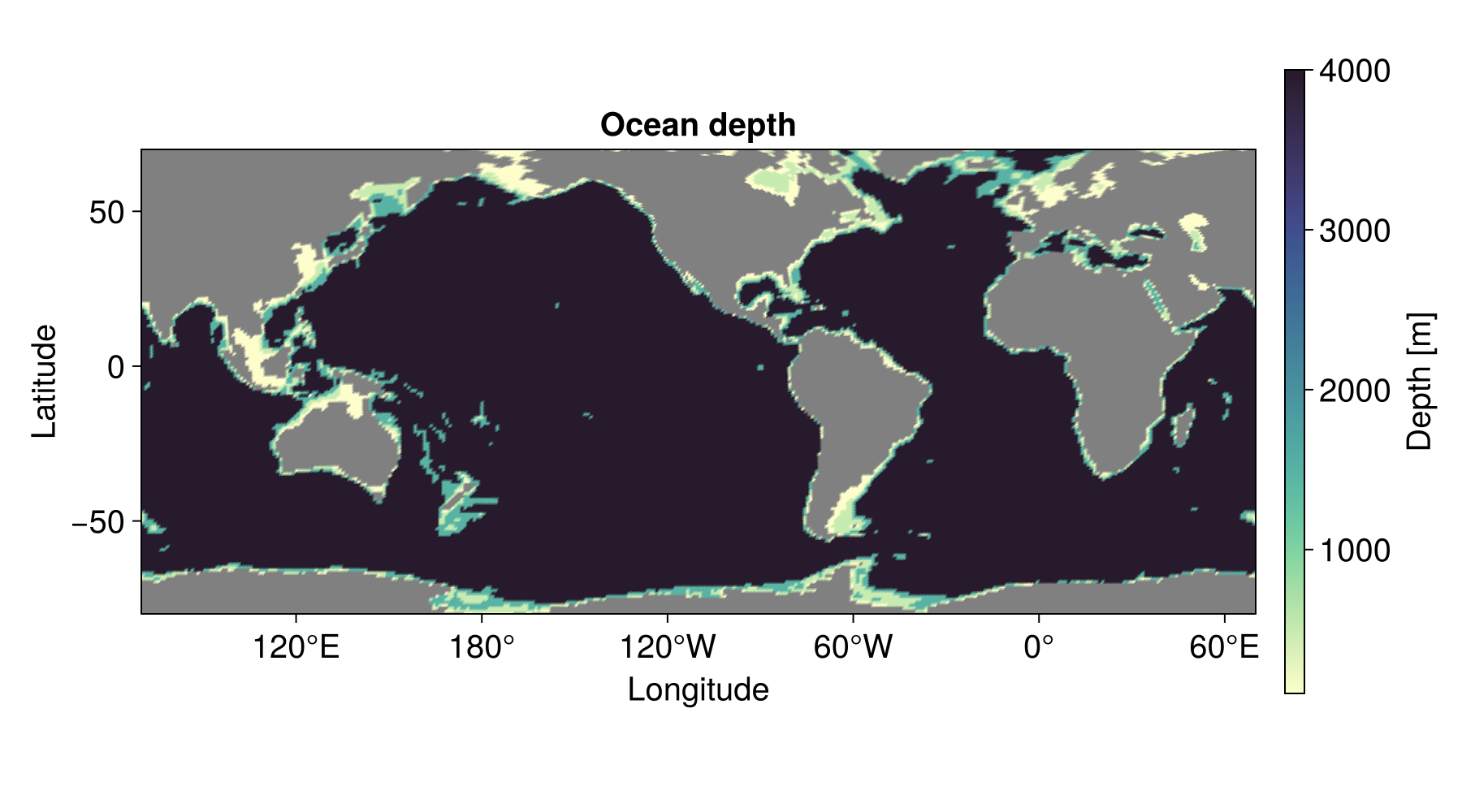
Wind stress and bottom drag
The zonal wind stress is a sum of four Gaussian wind belts,
the easterly trade winds and the westerlies of each hemisphere, whose strengths and latitudes follow the observed annual- and zonal-mean wind stress over the ocean from the NCEP/NCAR reanalysis. The trades overlap into weak easterlies on the equator, and the westerlies are almost three times stronger over the Southern Ocean than in the north. The curl drives cyclonic tropical and subpolar gyres and anticyclonic subtropical gyres, whose western boundary currents are the Gulf Stream and the Kuroshio. A positive flux boundary condition transports momentum out of the domain, so the momentum flux from the wind is minus the wind stress divided by the reference density ρ₀.
wind_belts = (northern_trades = FT(-0.055), southern_trades = FT(-0.065),
              northern_westerlies = FT(0.07), southern_westerlies = FT(0.19)) # [N m⁻²]
ρ₀ = 1020 # reference density [kg m⁻³]

wind_belt(φ, τ, φ₀) = τ * exp(-((φ - φ₀) / 11)^2)

zonal_wind_stress(φ, belts) = wind_belt(φ, belts.northern_trades, 18) + wind_belt(φ, belts.southern_trades, -17) +
                              wind_belt(φ, belts.northern_westerlies, 46) + wind_belt(φ, belts.southern_westerlies, -51)

zonal_momentum_flux(λ, φ, t, parameters) = - zonal_wind_stress(φ, parameters.wind_belts) / parameters.ρ₀
zonal_momentum_flux (generic function with 1 method)We plot the wind stress together with the Sverdrup transport per unit zonal width that it drives at Earth's rotation rate. The wind stress curl is
R = Oceananigans.defaults.planet_radius
Ω = Oceananigans.defaults.planet_rotation_rate

wind_stress_curl(φ) = - (zonal_wind_stress(φ + 0.01, wind_belts) - zonal_wind_stress(φ - 0.01, wind_belts)) / (R * deg2rad(0.02))
sverdrup_transport(φ, rotation_rate) = wind_stress_curl(φ) / (ρ₀ * 2 * rotation_rate * cosd(φ) / R)

latitudes = -80:0.5:80

fig = Figure(size=(800, 300))
ax = Axis(fig[1, 1], xlabel="Latitude [°]", ylabel="Zonal wind stress [N m⁻²]")
lines!(ax, latitudes, [zonal_wind_stress(φ, wind_belts) for φ in latitudes])
ax = Axis(fig[1, 2], xlabel="Latitude [°]", ylabel="Sverdrup transport [m² s⁻¹]")
lines!(ax, latitudes[abs.(latitudes) .> 5], sverdrup_transport.(latitudes[abs.(latitudes) .> 5], Ω))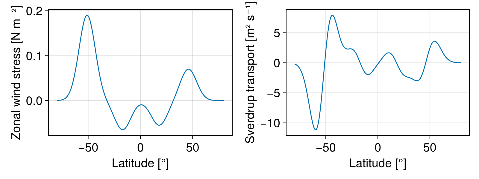
The wind stress enters through the top boundary condition on u. A quadratic BulkDrag acts on the sea floor, which is the bottom of the domain in the deep ocean and an immersed boundary everywhere else.
wind_stress = FluxBoundaryCondition(zonal_momentum_flux, parameters=(; wind_belts, ρ₀))
drag = BulkDrag(coefficient=FT(2.5e-3))
u_boundary_conditions = FieldBoundaryConditions(top=wind_stress, bottom=drag, immersed=ImmersedBoundaryCondition(bottom=drag))
v_boundary_conditions = FieldBoundaryConditions(bottom=drag, immersed=ImmersedBoundaryCondition(bottom=drag))
Oceananigans.FieldBoundaryConditions, with boundary conditions
├── west: DefaultBoundaryCondition (FluxBoundaryCondition: Nothing)
├── east: DefaultBoundaryCondition (FluxBoundaryCondition: Nothing)
├── south: DefaultBoundaryCondition (FluxBoundaryCondition: Nothing)
├── north: DefaultBoundaryCondition (FluxBoundaryCondition: Nothing)
├── bottom: FluxBoundaryCondition: BulkDragFunction(QuadraticFormulation(), Nothing, Cᴰ=0.0025)
├── top: DefaultBoundaryCondition (FluxBoundaryCondition: Nothing)
└── immersed: ImmersedBoundaryCondition with west=Nothing, east=Nothing, south=Nothing, north=Nothing, bottom=Flux, top=NothingSurface temperature restoring
The surface layer is restored on a 30-day time scale to
restoring_temperature(φ) = 30 * cosd(φ)^2

@inline function temperature_flux(i, j, grid, clock, fields, parameters)
    φ = φnode(i, j, grid.Nz, grid, Center(), Center(), Center())
    return @inbounds parameters.rate * (fields.T[i, j, grid.Nz] - restoring_temperature(φ))
end

restoring_rate = FT(100 / 30days) # surface layer thickness over the restoring time scale [m s⁻¹]
temperature_restoring = FluxBoundaryCondition(temperature_flux; discrete_form=true, parameters=(; rate=restoring_rate))
T_boundary_conditions = FieldBoundaryConditions(top=temperature_restoring)
Oceananigans.FieldBoundaryConditions, with boundary conditions
├── west: DefaultBoundaryCondition (FluxBoundaryCondition: Nothing)
├── east: DefaultBoundaryCondition (FluxBoundaryCondition: Nothing)
├── south: DefaultBoundaryCondition (FluxBoundaryCondition: Nothing)
├── north: DefaultBoundaryCondition (FluxBoundaryCondition: Nothing)
├── bottom: DefaultBoundaryCondition (FluxBoundaryCondition: Nothing)
├── top: FluxBoundaryCondition: DiscreteBoundaryFunction temperature_flux with parameters (rate=3.85802e-5,)
└── immersed: DefaultBoundaryCondition (FluxBoundaryCondition: Nothing)Free surface and time stepping
The barotropic gravity wave speed Δt, the free surface computes the number of substeps that keeps the barotropic CFL number at 0.7.
Δt = 1hour
free_surface = SplitExplicitFreeSurface(grid; cfl=0.7, fixed_Δt=Δt)
SplitExplicitFreeSurface substepping with FixedSubstepNumber(79)The model
We use WENO advection schemes for momentum and for temperature. Temperature sets the buoyancy through a linear equation of state. It starts from a horizontally uniform exponential thermocline with a 1 kilometer scale: a meridional density gradient across a basin comes with a depth-integrated thermal wind of hundreds of Sverdrups that would swamp the wind-driven gyres and take years to adjust away, so the equator-to-pole contrast enters only through the surface restoring.
momentum_advection = WENOVectorInvariant(order=5)
tracer_advection = WENO(order=7)
buoyancy = SeawaterBuoyancy(equation_of_state=LinearEquationOfState(thermal_expansion=2e-4), constant_salinity=35)
SeawaterBuoyancy{Float32}:
├── gravitational_acceleration: 9.80665
├── constant_salinity: 35.0
└── equation_of_state: LinearEquationOfState(thermal_expansion=0.0002, haline_contraction=0.00078)Poleward of about 60°, the restoring cools the surface below the water underneath it. A hydrostatic model cannot overturn such a column, so a convective adjustment mixes temperature and momentum vertically wherever the stratification is unstable.
closure = ConvectiveAdjustmentVerticalDiffusivity(convective_κz=1, convective_νz=1)

function build_model(grid, coriolis)
    model = HydrostaticFreeSurfaceModel(grid; coriolis, free_surface, buoyancy, closure,
                                        momentum_advection, tracer_advection,
                                        tracers = :T,
                                        timestepper = :SplitRungeKutta3,
                                        vertical_coordinate = ZStarCoordinate(),
                                        boundary_conditions = (u=u_boundary_conditions, v=v_boundary_conditions, T=T_boundary_conditions))

    set!(model, T = (λ, φ, z) -> 10 * exp(z / 1000))

    return model
end
build_model (generic function with 1 method)Three Coriolis parameters
The Coriolis parameter is the only thing that differs between the runs. Two of them use the spherical FPlane with the value of
The simulation runner saves the barotropic streamfunction
year = 365days

function run_gyres(grid, coriolis, name; stop_time=6year, save_interval=10days)
    model = build_model(grid, coriolis)
    simulation = Simulation(model; Δt, stop_time)

    wall_clock = Ref(time_ns())

    function progress(sim)
        u, v, w = sim.model.velocities
        elapsed = 1e-9 * (time_ns() - wall_clock[])
        @info @sprintf("%s, iter: %d, time: %s, max|u|: %.2f m/s, wall time: %s",
                       name, iteration(sim), prettytime(sim), maximum(abs, u), prettytime(elapsed))
        wall_clock[] = time_ns()
        return nothing
    end

    add_callback!(simulation, progress, IterationInterval(500))

    u, v, w = model.velocities
    U = Field(Integral(u, dims=3))
    ψ = Field(CumulativeIntegral(-U, dims=2))
    speed = Field(@at (Center, Center, Center) sqrt(u^2 + v^2))
    surface_speed = view(speed, :, :, grid.Nz)
    surface_temperature = view(model.tracers.T, :, :, grid.Nz)

    filename = "global_wind_driven_gyres_$name.jld2"

    simulation.output_writers[:surface] = JLD2Writer(model, (; ψ, surface_speed, surface_temperature); filename,
                                                     schedule = TimeInterval(save_interval),
                                                     array_type = Array{Float32},
                                                     overwrite_files = true)

    run!(simulation)

    return filename
end

rotation_rates = (Ω, Ω / 2)
coriolis_titles = Dict(Ω => "f = 2Ω sin φ", Ω / 2 => "f = Ω sin φ")
filenames = Dict(rotation_rate => run_gyres(grid, HydrostaticSphericalCoriolis(; rotation_rate, scheme=DualGridScheme(grid)), @sprintf("omega_%g", rotation_rate / Ω))
                 for rotation_rate in rotation_rates)

f_plane_filename = run_gyres(grid, FPlane(latitude=30, scheme=DualGridScheme(grid)), "f_plane")"global_wind_driven_gyres_f_plane.jld2"Gyre transports
The transport of a gyre is the difference between the streamfunction at the gyre center and on the coast, so we measure it as the range of
ψt = FieldTimeSeries(filenames[Ω], "ψ")
times = ψt.times

function gyre_transport(ψ, box)
    inside = @. (box.longitude[1] < mod(λ, 360) < box.longitude[2]) & (box.latitude[1] < φ < box.latitude[2])
    values = interior(ψ, :, :, 1)[inside]
    return maximum(values) - minimum(values)
end

gulf_stream = (longitude = (275, 310), latitude = (20, 42))
kuroshio = (longitude = (118, 160), latitude = (20, 42))
(longitude = (118, 160), latitude = (20, 42))Now we compare the transport time series at the two rotation rates.
Sv = 1e6 # m³ s⁻¹

fig = Figure(size=(900, 400))
axes = (gulf_stream = Axis(fig[1, 1], title="Gulf Stream", xlabel="Time [years]", ylabel="Transport [Sv]"),
        kuroshio = Axis(fig[1, 2], title="Kuroshio", xlabel="Time [years]"))

colors = Dict(zip(rotation_rates, Makie.wong_colors()))

for rotation_rate in rotation_rates
    streamfunctions = FieldTimeSeries(filenames[rotation_rate], "ψ")
    label = coriolis_titles[rotation_rate]
    color = colors[rotation_rate]

    for (name, box) in ((:gulf_stream, gulf_stream), (:kuroshio, kuroshio))
        transport = [gyre_transport(streamfunctions[n], box) for n in 1:length(times)]
        lines!(axes[name], times / year, transport / Sv; label, color)
    end
end

axislegend(axes.gulf_stream, position=:lt)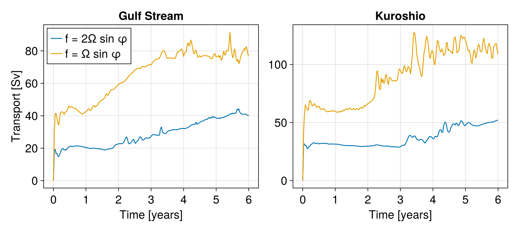
Halving the rotation rate roughly doubles the transport of both boundary currents.
The gyres
Next we plot the streamfunction at the end of each simulation. The Antarctic Circumpolar Current puts a large offset between
north_america = argmin(@. (mod(λ, 360) - 260)^2 + (φ - 40)^2)

function streamfunction_map!(fig, row, filename; title, colorrange)
    streamfunctions = FieldTimeSeries(filename, "ψ")
    ψ_end = interior(streamfunctions[end], :, :, 1)
    streamfunction = ifelse.(land, NaN, (ψ_end .- ψ_end[north_america]) / Sv)
    axis = map_axis(fig[row, 1]; title)
    sf = surface!(axis, λ, φ, 0 * λ; color=streamfunction, colormap=:balance, colorrange,
                  shading=NoShading, nan_color=:gray)
    Colorbar(fig[row, 2], sf, label="Streamfunction [Sv]")
    return nothing
end

experiments = ((filenames[Ω], coriolis_titles[Ω], (-100, 100)),
               (filenames[Ω / 2], coriolis_titles[Ω / 2], (-100, 100)),
               (f_plane_filename, "f = 2Ω sin 30°", (-1000, 1000)))

fig = Figure(size=(900, 1050))

for (row, (filename, title, colorrange)) in enumerate(experiments)
    streamfunction_map!(fig, row, filename; title, colorrange)
end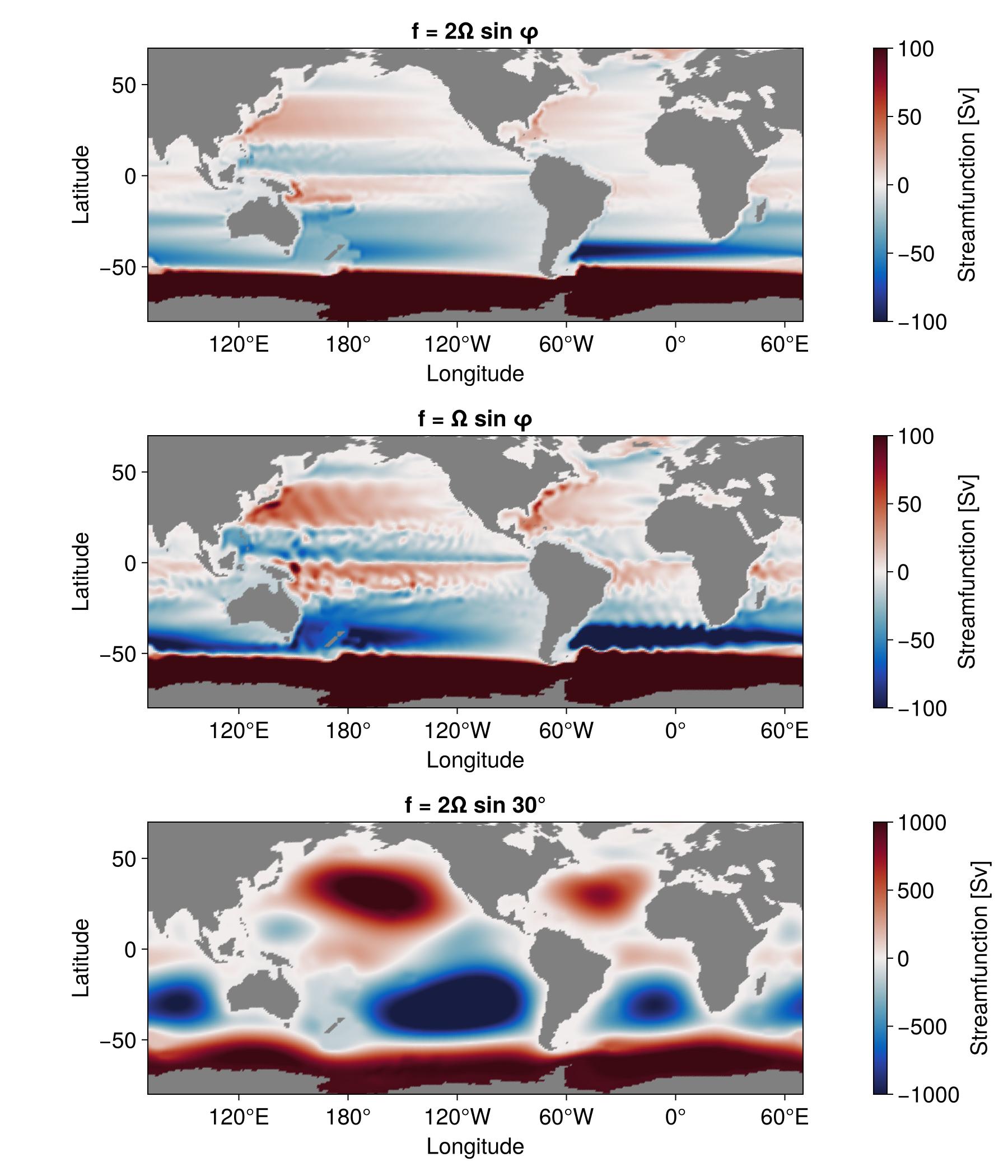
Halving the rotation rate doubles the gyres but leaves their shape alone: the streamfunction climbs to the gyre maximum within a few degrees of the western coast and decays slowly across the rest of the basin. On the
Currents and temperature
Finally we animate the global surface speed and, zoomed on the Gulf Stream and the Kuroshio, the departure of the surface temperature from its restoring profile,
restoring_profile = restoring_temperature.(φ)

gulf_stream_view = (limits = ((260, 320), (15, 55)), xticks = (270:15:315, ["90°W", "75°W", "60°W", "45°W"]))
kuroshio_view = (limits = ((115, 175), (15, 55)), xticks = (120:15:165, ["120°E", "135°E", "150°E", "165°E"]))

tripolar_grid = TripolarGrid(CPU(), Float64; size=(Nx, Ny, 1), z=(0, 1)) ## the regridder needs Float64 coordinates

latitude_longitude_grid((longitude, latitude)) =
    LatitudeLongitudeGrid(CPU(), Float64; longitude, latitude, topology=(Bounded, Bounded, Flat),
                          size=(2 * (longitude[2] - longitude[1]), 2 * (latitude[2] - latitude[1])))

regions = ("Gulf Stream" => gulf_stream_view, "Kuroshio" => kuroshio_view)
regional_grids = [latitude_longitude_grid(zoom.limits) for (_, zoom) in regions]
regridders = [ConservativeRegridding.Regridder(grid, tripolar_grid) for grid in regional_grids]

function regrid_temperature_anomaly(temperatures)
    anomaly = Field{Center, Center, Nothing}(tripolar_grid)
    regional_anomalies = [FieldTimeSeries{Center, Center, Nothing}(grid, temperatures.times) for grid in regional_grids]

    for n in eachindex(temperatures.times)
        set!(anomaly, ifelse.(land, NaN, interior(temperatures[n], :, :, 1) .- restoring_profile))
        for (anomalies, regridder) in zip(regional_anomalies, regridders)
            ConservativeRegridding.regrid!(anomalies[n], regridder, anomaly)
        end
    end

    return regional_anomalies
end

n = Observable(1)

fig = Figure(size=(1800, 1000))
Label(fig[1, 1:5], @lift(@sprintf("After %.1f years", times[$n] / year)); fontsize=22, tellwidth=false)

for (row, (filename, title, _)) in enumerate(experiments)
    speeds = FieldTimeSeries(filename, "surface_speed")
    speed = @lift ifelse.(land, NaN, interior(speeds[$n], :, :, 1))

    ax = map_axis(fig[row + 1, 1]; title="Surface speed, " * title)
    sf = surface!(ax, λ, φ, 0 * λ; color=speed, colormap=:magma, colorrange=(0, 0.3),
                  shading=NoShading, nan_color=:gray)
    row == 1 && Colorbar(fig[2:4, 2], sf, label="Speed [m s⁻¹]")

    regional_anomalies = regrid_temperature_anomaly(FieldTimeSeries(filename, "surface_temperature"))

    for (column, ((region, zoom), anomalies)) in enumerate(zip(regions, regional_anomalies))
        ax = map_axis(fig[row + 1, column + 2]; title="T − T*, $region, " * title, zoom...)
        sf = heatmap!(ax, @lift(anomalies[$n]); colormap=:balance, colorrange=(-2, 2), nan_color=:gray)
        row == 1 && column == 2 && Colorbar(fig[2:4, 5], sf, label="T − T* [°C]")
    end
end

CairoMakie.record(fig, "global_wind_driven_gyres.mp4", 1:2:length(times), framerate=12) do frame
    n[] = frame
end
┌ Warning: Assignment to `ax` in soft scope is ambiguous because a global variable by the same name exists: `ax` will be treated as a new local. Disambiguate by using `local ax` to suppress this warning or `global ax` to assign to the existing global variable.
└ @ ~/Oceananigans.jl-34546/docs/src/literated/global_wind_driven_gyres.md:39
┌ Warning: Assignment to `sf` in soft scope is ambiguous because a global variable by the same name exists: `sf` will be treated as a new local. Disambiguate by using `local sf` to suppress this warning or `global sf` to assign to the existing global variable.
└ @ ~/Oceananigans.jl-34546/docs/src/literated/global_wind_driven_gyres.md:40Julia version and environment information
This example was executed with the following version of Julia:
using InteractiveUtils: versioninfo
versioninfo()
Julia Version 1.13.0
Commit d1c37793dd2 (2026-09-09 19:00 UTC)
Build Info:
Official https://julialang.org release
Platform Info:
OS: Linux (x86_64-linux-gnu)
CPU: 128 × AMD EPYC 9374F 32-Core Processor
WORD_SIZE: 64
LLVM: libLLVM-20.1.8 (ORCJIT, znver4)
GC: Built with stock GC
Threads: 1 default, 1 interactive, 1 GC (on 128 virtual cores)
Environment:
JULIA_LOAD_PATH = @:@v#.#:@stdlib
JULIA_DEPOT_PATH = /var/lib/buildkite-agent/.julia:/var/lib/buildkite-agent/.julia/juliaup/julia-1.13.0+0.x64.linux.gnu/local/share/julia:/var/lib/buildkite-agent/.julia/juliaup/julia-1.13.0+0.x64.linux.gnu/share/julia
JULIA_VERSION_ENZYME = 1.13.0
JULIA_PKG_SERVER_REGISTRY_PREFERENCE = eager
LD_LIBRARY_PATH =
JULIA_MAX_NUM_PRECOMPILE_FILES = 24
JULIA_VERSION = 1.13.0
JULIA_CUDA_USE_COMPAT = false
JULIA_PROJECT = /var/lib/buildkite-agent/Oceananigans.jl-34546/docs/
JULIA_DEBUG = LiterateThese were the top-level packages installed in the environment:
import Pkg
Pkg.status()
Status `~/Oceananigans.jl-34546/docs/Project.toml`
[79e6a3ab] Adapt v4.7.3
⌃ [052768ef] CUDA v5.11.3
[13f3f980] CairoMakie v0.15.15
[8e50ac2c] ConservativeRegridding v0.2.15
⌅ [e30172f5] Documenter v1.17.0
[daee34ce] DocumenterCitations v1.5.0
[4710194d] DocumenterVitepress v0.3.7
[7da242da] Enzyme v0.13.214
[033835bb] JLD2 v0.6.7
[63c18a36] KernelAbstractions v0.9.44
[98b081ad] Literate v2.21.0
[da04e1cc] MPI v0.20.27
[85f8d34a] NCDatasets v0.14.15
[9e8cae18] Oceananigans v0.113.6 `..`
[429524aa] Optim v2.3.2
[f27b6e38] Polynomials v4.1.3
[3c362404] Reactant v0.2.291
[6038ab10] Rotations v1.7.1
[d496a93d] SeawaterPolynomials v0.3.11
[09ab397b] StructArrays v0.7.3
[bdfc003b] TimesDates v0.3.3
⌃ [0a941bbe] Zarr v0.10.2
[b77e0a4c] InteractiveUtils v1.11.0
[37e2e46d] LinearAlgebra v1.13.0
[44cfe95a] Pkg v1.13.0
Info Packages marked with ⌃ and ⌅ have new versions available. Those with ⌃ may be upgradable, but those with ⌅ are restricted by compatibility constraints from upgrading. To see why use `status --outdated`This page was generated using Literate.jl.